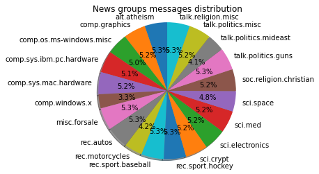
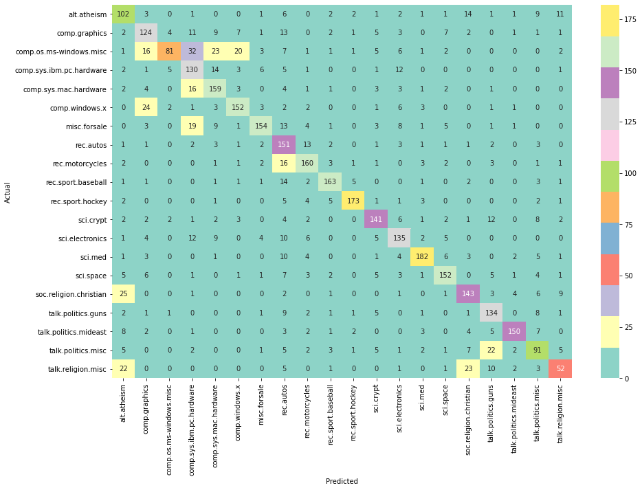
class: title-slide .row[ .col-7[ .title[ # News Groups ] .subtitle[ ## Exploring News Groups dataset ] .author[ ### Laxmikant Soni <br> [Web-Site](https://laxmikants.github.io) <br> [<i class="fab fa-github"></i>](https://github.com/laxmiaknts) [<i class="fab fa-twitter"></i>](https://twitter.com/laxmikantsoni09) ] .affiliation[ ] ] .col-5[ .logo[ <!-- --> ] Slides:<br> [laxmikants.github.io/datasets/slides](https://laxmikants.github.io/datasets/slides/NewsGroupsAnalysis.html#1) Materials:<br> [github.com/laxmikants/datasets](https://github.com/laxmikants/datasets) ] ] --- class: inverse, center, middle # The Newsgroups data set presents the problem of building a classifier that uses newsgroups posts to predict if a given article belongs to one of the 20 newsgroups (target_names). --- class: inverse, center, middle # Getting the Dataset --- class: body # 1. Getting the dataset ### 1.1 Fetch the dataset <hr> -- .pull-left[ [1] from sklearn.datasets import fetch_20newsgroups [2] dataset_full = fetch_20newsgroups(subset='all', remove=('headers', 'footers', 'quotes'), shuffle=True, random_state=42) [3] dataset_full.keys() [4] newsgroups_full.target_names ] -- .pull-right[ 'alt.atheism', 'comp.graphics', 'comp.os.ms-windows.misc', 'comp.sys.ibm.pc.hardware', 'comp.sys.mac.hardware', 'comp.windows.x' ... ] <hr> > `Newsgroups`: The 20 newsgroups dataset comprises around 18000 newsgroups posts on 20 topics --- class: inverse, center, middle # What's stored in the Dataset --- class: body # 2. What's stored in the Dataset ###2.1 What are the different values inside the dataset ? <hr> -- .pull-left[ [1] dir(dataset_full) [1] dataset_full.keys() [2] dataset_full['target_names'] [3] dataset_full['target'] [4] dataset_full['file_names'] ] -- .pull-right[ ['DESCR', 'data', 'filenames', 'target', 'target_names'] alt.atheism', 'comp.graphics', 'comp.os.ms-windows.misc target: 0, 1, 2, 3, 4, 5, 6, 7, 8, 9, 10, 11, 12, 13, 14, 15, 16, 17, 18, 19 C:\\Users\\slaxm\\scikit_learn_data\\20news_home\\20news-bydate-train\\rec.autos\\102994 -- ] <hr> > `keys`: different identification keys for fetching the details > `target_names`: different categories in which data is stored > `target`: 20 different unique index corresponding to target_names > `data`: actual daa is stored in different files having some `file_names` --- class: body # 2. What's stored in the Dataset...cont ###2.2 Print sample article from the newsgroup dataset ? <hr> -- .pull-left[ [1] dataset_full.data\[0\] [2] dataset_full.target\[0\] [3] dataset_full.target_names\[dataset_full.target\[0\]\] ] -- .pull-right[ `data` From: lerxst@wam.umd.edu (where's my thing)\nSubject: WHAT car is this!?\nNntp-Posting-Host: rac3.wam.umd.edu\nOrganization: University of Maryland, College Park\nLines: 15\n\n I was wondering if anyone out there could enlighten me on this car I saw\nthe other day. It was a 2-door sports car, looked to be from the late 60s/\nearly 70s. It wa `target` 7 `target_name` rec.autos ] <hr> The first document is from the `rec.autos` newsgroup, which was assigned the number `7`. Reading this post, we can easily figure out it's about cars. The word car actually occurs a number of times in the document. Words such as bumper also seem very car-oriented --- class: inverse, center, middle # cleaning the data --- class: body # 3. cleaning the data (Stemming and lemmatizing).. cont ###3.1 Split textual data into smaller and more meaningful components called tokens -- .pull-left[ [1] def `normal_tokenizer(str_input)`: [2] words = re.sub(r"\[^A-Za-z\-\]", " ", str_input).lower().split() [3] return words ] -- .pull-right[ text = "A \ letter 09 words having a84 kind * 1234 and other stuff" will get converted to \['a', 'letter', 'words', 'having', 'a', 'kind', 'and', 'other', 'stuff'\] ] -- <hr> > `normal_tokenizer` removes non english characters and alpha numeric words and split them on spaces --- class: body # 3. cleaning the data (Stemming and lemmatizing).. cont ### 3.2 Remove all the endings from the words to get base form of the word -- .pull-left[ [1] def `stem_tokenizer(str_input)`: [2] words = re.sub(r"[^A-Za-z]", " ", str_input).lower().split() [3] words = [porter_stemmer.stem(word) for word in words if len(word) > 2] [4] return words ] -- .pull-right[ text = "A \ letter 09 words having a84 kind * 1234 and other stuff" will get converted to ['letter', 'word', 'have', 'kind', 'and', 'other', 'stuff'] ] -- ] <hr> > `stem_tokenizer` keeps only words having more than two characters > `stem_tokenizer` strips the endings off of words --- class: body # 3. cleaning the data (Stemming and lemmatizing).. cont ###3.3 Get the root form of the word present in the dictionary using lemmatization -- .pull-left[ [1] lemmatizer = `WordNetLemmatizer()` [2] def `lemma_tokenizer`(str_input): [3] words = re.sub(r"\[^A-Za-z\]", " ", str_input).lower().split() [4] words = \[lemmatizer.`lemmatize(word)` for word in words if len(word) > 2 and word in validwords\] [5] return words ] -- .pull-right[ text = "A \ letter 09 words having a84 kind * 1234 and other stuff" will get converted to ['letter', 'word', 'have', 'kind', 'and', 'other', 'stuff'] ] -- ] <hr> > `lemma_tokenizer` keeps only words having more than two characters > `lemma_tokenizer` guarantees to return a valid word --- class: inverse, center, middle # Exploring the newsgroup dataset --- class: body # 4 Exploring the Dataset ### Show the plot of how the data is structured ? <hr> -- .pull-left[ [1] import seaborn as sns [2] import matplotlib.pyplot as plt [3] sns.distplot(dataset_full.target) [4] plt.show() ] -- .pull-right[ <!-- --> ] `distribution:` It is good to visualize to get a general idea of how the data is structured --- class: body # 4 Exploring the Dataset (Pie chart distribution) ### Show the pie chart of the newsgroup distribution ? <hr> -- .pull-left[ [1] labels = newsgroups_full\.target_names [2] slices = \[\] [3] for key in newsgroups\_full\_dnry: slices.append(newsgroups_full_dnry[key]) [4] fig , ax = plt.subplots() [5] ax.pie(slices, labels = labels , autopct = '%1.1f%%', shadow = True, startangle = 90) ] -- .pull-right[ <!-- --> ] <hr> `Pie Distribution:` It is better to view relative distribution of articles as pie chart --- class: body # 4 Exploring the Dataset ### What is newsgroup wise count of words ? <hr> -- .pull-left[ [1] for ind in range(len(newsgroups\_full.data)): [2] grp_name = newsgroups\_full.target_names\[newsgroups_full.target\[ind\]] [3] if grp\_name in newsgroups\_full\_dnry: [4] newsgroups\_full\_dnry\[grp_name\] += 1 [5] else: [6] newsgroups\_full\_dnry\[grp_name\] = 1 ] -- .pull-right[ Total number of articles in dataset 18846 Number of articles category wise: {'rec.sport.hockey': 999, 'comp.sys.ibm.pc.hardware': 982, 'talk.politics.mideast': 940, 'comp.sys.mac.hardware': 963, 'sci.electronics': 984, 'talk.religion.misc': 628, 'sci.crypt': 991, 'sci.med': 990, 'alt.atheism': 799, 'rec.motorcycles': 996, 'rec.autos': 990, 'comp.windows.x': 988, 'comp.graphics': 973 ] <hr> `Word count:` A simple word count category wise gives general idea about what people are posting --- class: inverse, center, middle # Feature extraction --- class: body # 5. Feature extraction ### What are the feature in the newsgroups dataset ? <hr> -- .pull-left[ [1] from sklearn.feature_extraction_text import CountVectorizer [2] count_vectorizer = CountVectorizer(stop_words='english', tokenizer = lemma_tokenizer) [3] extracted = count_vectorizer.fit_transform(dataset_full.data) [4] extracted.get_feature_names() ] -- .pull-right[ 'car' : 1147, 'like' : 356, 'ani' : 353, 'use' : 344, 'know' : 252, 'drive': 235, 'think': 229, 'new' : 227, 'good' : 222, 'time' : 219, 'veri' : 207, 'look' : 205, 'year' : 199, ] <hr> `feature engineering`: The variable being predicted is referred to by a number of different names, such as target, label, and outcome. The variables being used to make the predictions are variously called predictors, regressors, features, and attributes.Determining what attributes to use for making predictions is called feature engineering. --- class: inverse, center, middle # Creating text classifier --- class: body # 6. Creating text classifer ### 6.1. Split the data in training and testing set <hr> -- .pull-left[ [1] from sklearn.model\_selection import train\_test\_split [2] import numpy as np [3] X\_train, X\_test, Y\_train_source, Y\_test_source, train\_source\_names, test\_source\_names = train\_test\_split(np.array(newsgroups\_full\_df\['clean_text'\]), np.array(newsgroups_full_df\['source'\]),np.array(newsgroups\_full\_df['source\_name']), test\_size=0.33, random\_state=42) [4] X_train.shape, X_test.shape ] -- .pull-right[ | source_name | train_count | test_count | |--------------------------|-------------|------------| | rec.sport.baseball | 693 | 301 | | sci.space | 670 | 317 | | comp.os.ms-windows.misc | 669 | 316 | | comp.sys.ibm.pc.hardware | 667 | 315 | ] <hr> `train_test_split`:We need to randomly split the original dataset into two sets, the training and testing sets, which simulate learning data and prediction data respectively. Generally, the proportion of the original dataset to include in the testing split can be 25%, 33.3%, or 40%. We use the train\_test\_split function from scikit-learn to do the random splitting and to preserve the percentage of samples for each class --- class: body # 6. Creating text classifer ###6.2. Build the MultiNomialNB classifier <hr> -- .pull-left[ [1] cv = CountVectorizer(stop\_words = 'english',binary=False, min_df=2, max_df= 0.95) cv\_train\_features = cv.fit\_transform(X\_train) [2] cv\_test\_features = cv.transform(X\_test) [3] mnb = MultinomialNB(alpha=.05) [4] mnb.fit(cv\_train\_features, train\_source\_names) ] -- .pull-right[ BOW model: Train features shape: (15076, 28489), Test features shape: (3770, 28489) ] <hr> `MultiNomialNB`:The multinomial Naive Bayes classifier is suitable for classification with discrete features (e.g., word counts). --- class: inverse, center, middle # Performance evaluation --- class: body # 7. Performance evaluation of the model ###7.1. What is the accuracy of the model ? <hr> -- .pull-left[ [1] mnb\_bow\_cv\_scores = cross\_val\_score(mnb, cv\_train\_features, train\_source\_names, cv=5) [2] mnb\_bow\_cv\_mean_score = np.mean(mnb\_bow\_cv\_scores) [3] mnb\_bow\_test\_score = mnb.score(cv\_test\_features, test\_source\_names) ] -- .pull-right[ CV Accuracy (5-fold): [0.72015915 0.71608624 0.72039801 0.72769486 0.70912106] Mean CV Accuracy: 0.7186918634062225 Test Accuracy: 0.7238726790450929 ] <hr> `Accuracy`: Accuracy is one metric for evaluating classification models. Accuracy is the fraction of predictions our model got right. --- class: body # 7. Performance evaluation of the model ###7.2 Draw the a confusion matrix of the model ? <hr> -- .pull-left[ [1] conf\_mat = confusion\_matrix(test\_source\_names, Y\_pred) [2] fig, ax = plt.subplots(figsize=(15, 10)) [3] sns.heatmap(conf_mat, annot=True, cmap = "Set3", fmt ="d", xticklabels=labels, yticklabels=labels) [4] plt.ylabel('Actual') [5] plt.xlabel('Predicted') [6] plt.show() ] -- .pull-right[ <!-- --> ] <hr> `Confusion matrix`: The heat map shows a confusion matrix. It is a good tool to evalute the performance of the model. --- class: inverse, center, middle # Thanks