EDA with Iris dataset
Exploring datasets is an important topic in data science. To achieve this task EDA i.e Exploratory data analysis helps
Loading the dataset
Exploring datasets is an important topic in data science. To achieve this task EDA i.e Exploratory data analysis helps by means of summary statistics and other infographics. In this post we will take iris dataset and apply EDA techiniqes to better gain an insight into the dataset.
from sklearn.datasets import load_iris


iris_dataset = load_iris()

print(type(iris_dataset))
## <class 'sklearn.utils.Bunch'>print(iris_dataset.keys())## dict_keys(['data', 'target', 'frame', 'target_names', 'DESCR', 'feature_names', 'filename'])The dataset is of Bunch datatypes having keys 'data', 'target', 'frame', 'target_names', 'DESCR', 'feature_names', 'filename'.
Before we go ahead we need to convert Bunch to pandas DataFrame.
creating dataframe from raw data
import pandas as pd

iris_df = pd.DataFrame(iris_dataset.data, columns = iris_dataset.feature_names)

print(iris_df.head())
## sepal length (cm) sepal width (cm) petal length (cm) petal width (cm)
## 0 5.1 3.5 1.4 0.2
## 1 4.9 3.0 1.4 0.2
## 2 4.7 3.2 1.3 0.2
## 3 4.6 3.1 1.5 0.2
## 4 5.0 3.6 1.4 0.2The columns shows the length, width but does not show the group to which this length or width belongs. The group to which these values belong is stored in target_names which can stored in seperate column in our dataframe as.
group_names = pd.Series([iris_dataset.target_names[ind] for ind in iris_dataset.target], dtype = 'category')

iris_df['group'] = group_names


print(iris_df.head())
## sepal length (cm) sepal width (cm) ... petal width (cm) group
## 0 5.1 3.5 ... 0.2 setosa
## 1 4.9 3.0 ... 0.2 setosa
## 2 4.7 3.2 ... 0.2 setosa
## 3 4.6 3.1 ... 0.2 setosa
## 4 5.0 3.6 ... 0.2 setosa
##
## [5 rows x 5 columns]Getting summary statistical measures
To start with EDA, mean and median should be calculated for the numeric variables. To get the summary statistics we use describe function.
iris_sumry = iris_df.describe().transpose()

iris_sumry['std'] = iris_df.std()

iris_sumry.head()
## count mean std min 25% 50% 75% max
## sepal length (cm) 150.0 5.843333 0.828066 4.3 5.1 5.80 6.4 7.9
## sepal width (cm) 150.0 3.057333 0.435866 2.0 2.8 3.00 3.3 4.4
## petal length (cm) 150.0 3.758000 1.765298 1.0 1.6 4.35 5.1 6.9
## petal width (cm) 150.0 1.199333 0.762238 0.1 0.3 1.30 1.8 2.5There is no feature which is having a mean as zero. The average sepal width and petal length are not much different. The median of petal length is much different from the mean.
For sepal length 25% quartile is 5.1 i.e 25% of the dataset values for this feature are less than 5.1
Checking skewness and kurtosis
To check whether the petal length is normaly distributed or not we find the skewness and kurtosis and perform the test as…
from scipy.stats import skew, skewtest

petal_length = iris_df['petal length (cm)']

sk = skew(petal_length)

z_score, p_value = skewtest(petal_length)

print('Skewness %0.3f z-score %0.3f p-value %0.3f' % (sk, z_score, p_value))
## Skewness -0.272 z-score -1.400 p-value 0.162
from scipy.stats import kurtosis, kurtosistest

petal_length = iris_df['petal length (cm)']

ku = kurtosis(petal_length)

z_score, p_value = kurtosistest(petal_length)

print('Kurtosis %0.3f z-score %0.3f p-value %0.3f' % (ku, z_score, p_value))
## Kurtosis -1.396 z-score -14.823 p-value 0.000From the values of skewness and kurtosis we see that the petal length of plants is skewed to the left.
Creating categorical dataframe
To create a categorical dataframe from the quantitative data we can make use of the binning as. Binning transforms the numeric data into categorical data. In EDA this helps in reducing outliers.
perct = [0,.25,.5,.75,1]

iris_bin = pd.concat(

    [pd.qcut(iris_df.iloc[:,0], perct, precision=1),

    pd.qcut(iris_df.iloc[:,1], perct, precision=1),

    pd.qcut(iris_df.iloc[:,2], perct, precision=1),

    pd.qcut(iris_df.iloc[:,3], perct, precision=1)],

    join='outer', axis = 1)
Frequencies and Contingency tables
The resulting frequencies of each class of species in iris dataset can be obtained as …
print(iris_df['group'].value_counts())## virginica 50
## versicolor 50
## setosa 50
## Name: group, dtype: int64The resultant frequencies for the binned dataframe
print(iris_bin['petal length (cm)'].value_counts())## (0.9, 1.6] 44
## (4.4, 5.1] 41
## (5.1, 6.9] 34
## (1.6, 4.4] 31
## Name: petal length (cm), dtype: int64We can describe the binned dataframe using the describe function
iris_bin.describe().transpose()## count unique top freq
## sepal length (cm) 150 4 (4.2, 5.1] 41
## sepal width (cm) 150 4 (1.9, 2.8] 47
## petal length (cm) 150 4 (0.9, 1.6] 44
## petal width (cm) 150 4 (0.0, 0.3] 41Contingency tables based on groups and binning can be obtained as…
print(pd.crosstab(iris_df['group'], iris_bin['petal length (cm)']))## petal length (cm) (0.9, 1.6] (1.6, 4.4] (4.4, 5.1] (5.1, 6.9]
## group
## setosa 44 6 0 0
## versicolor 0 25 25 0
## virginica 0 0 16 34Cross tabulation can further used to apply chi-square test to determine which feature has the effect on the species of the plant. Further chi-square test can help us understand the relationship between target outcome (plant group) and other independant variables (length and width). For example one can setup a chi-squre test to check if the petal length is statistically different from each other i.e values are significantly different across class of species.
Applying t-test to check statistical signifcance
from scipy.stats import ttest_ind

grp0 = iris_df['group'] == 'setosa'

grp1 = iris_df['group'] == 'versicolor'

grp2 = iris_df['group'] == 'virginica'

petal_length = iris_df['petal length (cm)']


print('var1 %0.3f var2 %03f' % (petal_length[grp1].var(),

                                petal_length[grp2].var()))
## var1 0.221 var2 0.304588sepal_width = iris_df['sepal width (cm)']
t, p_value = ttest_ind(sepal_width[grp1], sepal_width[grp2], axis=0, equal_var=False)
print('t statistic %0.3f p-value %0.3f' % (t, p_value))## t statistic -3.206 p-value 0.002The p-value shows that group means are significantly different.
Further we can check it among more than 2 groups using ANOVA
from scipy.stats import f_oneway

sepal_width = iris_df['sepal width (cm)']

f, p_value = f_oneway(sepal_width[grp0],

                     sepal_width[grp1],

                     sepal_width[grp2])

print('One-way ANOVA F-value %0.3f p-value %0.3f' % (f,p_value))
## One-way ANOVA F-value 49.160 p-value 0.000Applying chi-square to cagegorical variables
from scipy.stats import chi2_contingency

table = pd.crosstab(iris_df['group'],

                    iris_bin['petal length (cm)'])

chi2, p, dof, expected = chi2_contingency(table.values)

print('Chi-square %0.2f p-value %0.3f' % (chi2, p))
## Chi-square 212.43 p-value 0.000The p-value and chi-square value indicates that petal length variable can be effectively used for distinguishing between iris groups.
Visualising data
Creating box plot
import seaborn as sns

import matplotlib.pyplot as plt

sns.boxplot(x="group",y="petal length (cm)",data=iris_df)

plt.show()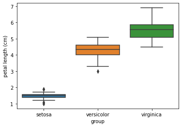
The box plot shows that the 3 groups, setosa, versicolor, and virginica, have different petal lengths.
Conclusion
In this artical we hv seen how to apply to do exploratary data analysis with iris dataset. We also learned the tools that help us understand the relationship between outcome variable and independent variables. We learned various techniqes in EDA that can be used before building the machine learning models.