Classification
Classifcation models a function to predict a specific outcome out of mulitple possible outcomes.
Classification
With regression we now predicted specific output-values for certain given input-values. Sometimes, however, we are not trying to predict outputs but to categorize or classify our elements. For this, we use classification algorithms
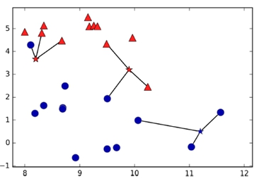
In the figure above, we see one specific kind of classification algorithm, namely the K-Nearest-Neighbor classifier. Here we already have a decent amount of classified elements. We then add a new one (represented by the stars) and try to predict its class by looking at its nearest neighbors.
CLASSIFICATION ALGORITHMS
There are various different classification algorithms and they are often used for predicting medical data or other real life use-cases. For example, by providing a large amount of tumor samples, we can classify if a tumor is benign or malignant with a pretty high certainty.
K-NEAREST-NEIGHBORS
As already mentioned, by using the K-Nearest-Neighbors classifier, we assign the class of the new object, based on its nearest neighbors. The K specifies the amount of neighbors to look at. For example, we could say that we only want to look at the one neighbor who is nearest but we could also say that we want to factor in 100 neighbors. Notice that K shouldn’t be a multiple of the number of classes since it might cause conflicts when we have an equal amount of elements from one class as from the other.
NAIVE-BAYES
The Naive Bayes algorithm might be a bit confusing when you encounter it the first time. However, we are only going to discuss the basics and focus more on the implementation in Python later on.
| Outlook | Temperture | Humidity | Windy | Play |
|---|---|---|---|---|
| Sunny | Hot | High | FALSE | No |
| Sunny | Hot | High | TRUE | No |
| Rainy | Mild | High | FALSE | No |
| Rainy | Hot | High | TRUE | No |
| Overcast | Hot | Normal | TRUE | Yes |
| Sunny | Hot | Normal | TRUE | Yes |
| Sunny | Mild | High | TRUE | Yes |
| Overcast | Cold | Normal | TRUE | No |
Imagine that we have a table like the one above. We have four input values (which we would have to make numerical of course) and one label or output. The two classes are Yes and No and they indicate if we are going to play outside or not.
What Naive Bayes now does is to write down all the probabilities for the individual scenarios. So we would start by writing the general probability of playing and not playing. In this case, we only play three out of eight times and thus our probability of playing will be 3/8 and the probability of not playing will be 5/8.
Also, out of the five times we had a high humidity we only played once, whereas out of the three times it was normal, we played twice. So our probability for playing when we have a high humidity is 1/5 and for playing when we have a medium humidity is 2/3. We go on like that and note all the probabilities we have in our table. To then get the classification for a new entry, we multiply the probabilities together and end up with a prediction.
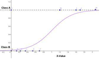
LOGISTIC REGRESSION
Another popular classification algorithm is called logistic regression . Even though the name says regression , this is actually a classification algorithm. It looks at probabilities and determines how likely it is that a certain event happens (or a certain class is the right one), given the input data. This is done by plotting something similar to a logistic growth curve and splitting the data into two.
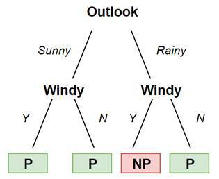
DECISION TREES
With decision tree classifiers, we construct a decision tree out of our training data and use it to predict the classes of new elements.
Since we are not using a line (and thus our model is not linear), we are also preventing mistakes caused by outliers.
This classification algorithm requires very little data preparation and it is also very easy to understand and visualize. On the other hand, it is very easy to be overfitting the model. Here, the model is very closely matched to the training data and thus has worse chances to make a correct prediction on new data.
RANDOM FOREST
Rndom forest classifier is based on decision trees. What it does is creating a forest of multiple decision trees. To classify a new object, all the various trees determine a class and the most frequent result gets chosen. This makes the result more accurate and it also prevents overfitting. It is also more suited to handle data sets with higher dimensions. On the other hand, since the generation of the forest is random , you have very little control over your model.
LOADING DATA
Now let us get into the code. In this example, we will get our data directly from the sklearn module. For the program we need the following imports:
import numpy as np
import pandas as pd
from sklearn.model_selection import train_test_split
from sklearn.neighbors import KNeighborsClassifier
from sklearn.datasets import load_breast_cancer
At the last import, we import a dataset containing data on breast cancer. Also notice that we are only importing the KNeighborsClassifier for now.
data = load_breast_cancer()
print (data.feature_names)
## ['mean radius' 'mean texture' 'mean perimeter' 'mean area'
## 'mean smoothness' 'mean compactness' 'mean concavity'
## 'mean concave points' 'mean symmetry' 'mean fractal dimension'
## 'radius error' 'texture error' 'perimeter error' 'area error'
## 'smoothness error' 'compactness error' 'concavity error'
## 'concave points error' 'symmetry error' 'fractal dimension error'
## 'worst radius' 'worst texture' 'worst perimeter' 'worst area'
## 'worst smoothness' 'worst compactness' 'worst concavity'
## 'worst concave points' 'worst symmetry' 'worst fractal dimension']print (data.target_names)## ['malignant' 'benign']targets, we have two options in this dataset: malignant and benign .
PREPARING DATA
Again, we convert our data back into NumPy arrays and split them into training and test data.
X = np.array(data.data)
Y = np.array(data.target)
X_train, X_test, Y_train, Y_test = train_test_split(X,Y, test_size = 0.1 )
The data attribute refers to our features and the target attribute points to the classes or labels. We again choose a test size of ten percent.
TRAINING AND TESTING
We start by first defining our K-Nearest-Neighbors classifier and then training it.
knn = KNeighborsClassifier( n_neighbors = 5 )
knn.fit(X_train, Y_train)
## KNeighborsClassifier()The n_neighbors parameter specifies how many neighbor points we want to consider. In this case, we take five. Then we test our model again for its accuracy.
accuracy = knn.score(X_test, Y_test)
print (accuracy)
## 0.9473684210526315We get a pretty decent accuracy for such a complex task.
0.9649122807017544
THE BEST ALGORITHM
Now let’s put all the classification algorithms that we’ve discussed up until now to use and see which one performs best.
from sklearn.neighbors import KNeighborsClassifier
from sklearn.naive_bayes import GaussianNB
from sklearn.linear_model import LogisticRegression
from sklearn.tree import DecisionTreeClassifier
from sklearn.ensemble import RandomForestClassifier
clf1 = KNeighborsClassifier( n_neighbors = 5 )
clf2 = GaussianNB()
clf3 = LogisticRegression()
clf4 = DecisionTreeClassifier()
clf5 = RandomForestClassifier()
clf1.fit(X_train, Y_train)## KNeighborsClassifier()clf2.fit(X_train, Y_train)## GaussianNB()clf3.fit(X_train, Y_train)## LogisticRegression()
##
## C:\Users\slaxm\AppData\Local\R-MINI~1\envs\R-RETI~1\lib\site-packages\sklearn\linear_model\_logistic.py:765: ConvergenceWarning: lbfgs failed to converge (status=1):
## STOP: TOTAL NO. of ITERATIONS REACHED LIMIT.
##
## Increase the number of iterations (max_iter) or scale the data as shown in:
## https://scikit-learn.org/stable/modules/preprocessing.html
## Please also refer to the documentation for alternative solver options:
## https://scikit-learn.org/stable/modules/linear_model.html#logistic-regression
## extra_warning_msg=_LOGISTIC_SOLVER_CONVERGENCE_MSG)clf4.fit(X_train, Y_train)## DecisionTreeClassifier()clf5.fit(X_train, Y_train)## RandomForestClassifier()print (clf1.score(X_test, Y_test))## 0.9473684210526315print (clf2.score(X_test, Y_test))## 0.9649122807017544print (clf3.score(X_test, Y_test))## 0.9649122807017544print (clf4.score(X_test, Y_test))## 0.9473684210526315print (clf5.score(X_test, Y_test))## 0.9824561403508771When you run this program a couple of times, you will notice that we can’t really say which algorithm is the best. Every time we run this script, we will see different results, at least for this specific data set.
PREDICTING LABELS
Again, we can again make predictions for new, unknown data. The chance of success in the classification is even very high. We just need to pass an array of input values and use the predict function .
X_new = np.array([[...]])
Y_new = clf.predict(X_new)