Logistic Regression in ML
Applying Logistic Regression to datasets

Logistic Regression
Introduction
Logistic regression is a machine learning classification algorithm. The algorithm assigns observations to a set of classes. The logistic regration is used to predict a categorical variabble.
Comparison to linear regression
If we are given dataset which contains study time and exam scrores. Then
- Linear Regression helps to predic the exam scroes which is a continuous variable.
- Logistic Regression can predict if the student passed or failed which is a discrete categorical variable
Types of logistic regression
- Binary (Pass/Fail)
- Multi (Cats, Dogs, Sheep)
- Ordinal (Low, Medium, High)
Binary logistic regression
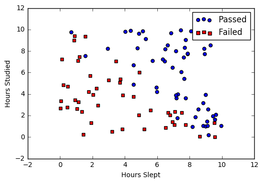
If we are having dataset of student exam results and the objective is to predict student will pass or faile based on hours slept and hours spent studying.
| Studied | Slept | Passed |
| 4.85 | 9.63 | 1 |
| 8.62 | 3.23 | 0 |
| 5.43 | 8.23 | 1 |
| 9.21 | 6.34 | 0 |
Graph of the data
image
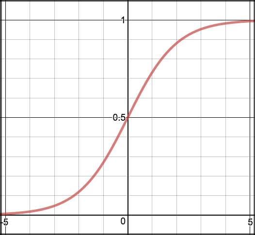
Sigmoid activation
Generally probability is assigned to predicted values. For this we use sigmoid function which maps predictions to probabilities.
Math
\[S(z) = \frac{1} {1 + e^{-z}}\]
note
- \(s(z)\) = output between 0 and 1 (probability estimate)
- \(z\) = input to the function (your algorithm’s prediction e.g. mx +
- \(e\) = base of natural log
Graph
image
Code
sigmoid <- function(z) {
#SIGMOID Compute sigmoid functoon
# J <- SIGMOID(z) computes the sigmoid of z.
# You need to return the following variables correctly
z <- as.matrix(z)
g <- matrix(0,dim(z)[1],dim(z)[2])
# ----------------------- YOUR CODE HERE -----------------------
# Instructions: Compute the sigmoid of each value of z (z can be a matrix,
# vector or scalar).
g <- 1 / (1 + exp(-1 * z))
g
# ----------------------------------------------------
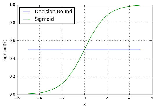
}Decision boundary
The prediction function returns probability value between 0 and 1. Map this to a discrete class (true/false) based on some threshold value.
\[p \geq 0.5, class=1 \\ p < 0.5, class=0\]
For example, if our threshold is .5 and our prediction function returned .7, we will classify this observation as positive. If our prediction is .1 we would classify the observation as negative.
image
Making predictions
To make predictions we need to find the probability of our observations.
Math
\[z = W_0 + W_1 Studied \]
We can transform the output using the sigmoid function to return a probability value between 0 and 1.
\[P(class=1) = \frac{1} {1 + e^{-z}}\]
If the model returns .3 it believes there is only a 30% chance of passing and this would be classified as fail.
Code
predict <- function(theta, X) {

  m <- dim(X)[1] # Number of training examples

  p <- rep(0,m)

  p[sigmoid(X %*% theta) >= 0.5] <- 1

  p
  # ----------------------------------------------------
}
A group of 20 students spend between 0 and 6 hours studying for an exam. How does the number of hours spent studying affect the probability that the student will pass the exam?
Hours <- c(0.50, 0.75, 1.00, 1.25, 1.50, 1.75, 1.75, 2.00, 2.25,
           2.50, 2.75, 3.00, 3.25, 3.50,    4.00,   4.25,   4.50,   4.75,
           5.00, 5.50)
Pass    <- c(0, 0, 0, 0, 0, 0, 1,   0, 1, 0, 1, 0, 1, 0, 1, 1, 1,   1, 1, 1)

HrsStudying <- data.frame(Hours, Pass)
The table shows the number of hours each student spent studying, and whether they passed (1) or failed (0).
HrsStudying_Table <- t(HrsStudying); HrsStudying_Table## [,1] [,2] [,3] [,4] [,5] [,6] [,7] [,8] [,9] [,10] [,11] [,12] [,13]
## Hours 0.5 0.75 1 1.25 1.5 1.75 1.75 2 2.25 2.5 2.75 3 3.25
## Pass 0.0 0.00 0 0.00 0.0 0.00 1.00 0 1.00 0.0 1.00 0 1.00
## [,14] [,15] [,16] [,17] [,18] [,19] [,20]
## Hours 3.5 4 4.25 4.5 4.75 5 5.5
## Pass 0.0 1 1.00 1.0 1.00 1 1.0The graph shows the probability of passing the exam versus the number of hours studying, with the logistic regression curve fitted to the data.
library(ggplot2)## Warning: package 'ggplot2' was built under R version 4.0.5ggplot(HrsStudying, aes(Hours, Pass)) +
geom_point(aes()) +
geom_smooth(method='glm', family="binomial", se=FALSE) +
labs (x="Hours Studying", y="Probability of Passing Exam",
title="Probability of Passing Exam vs Hours Studying")## Warning: Ignoring unknown parameters: family## `geom_smooth()` using formula 'y ~ x'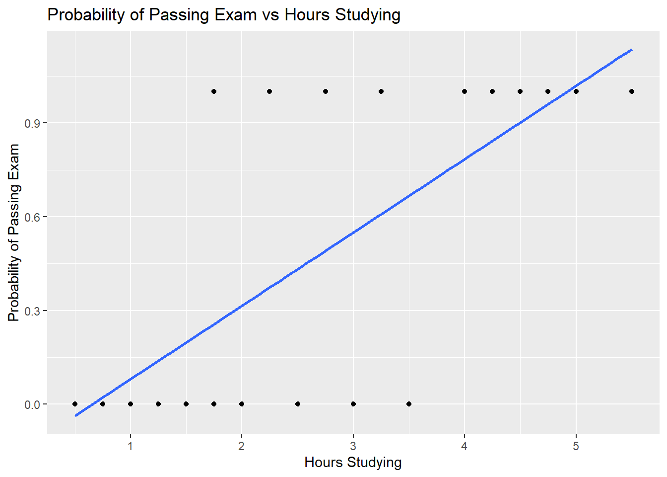 The logistic regression analysis gives the following output.
model <- glm(Pass ~.,family=binomial(link='logit'),data=HrsStudying)
model$coefficients
## (Intercept) Hours
## -4.077713 1.504645Coefficient Std.Error z-value P-value (Wald)
Intercept -4.0777 1.7610 -2.316 0.0206
Hours 1.5046 0.6287 2.393 0.0167
The output indicates that hours studying is significantly associated with the probability of passing the exam (p=0.0167, Wald test). The output also provides the coefficients for Intercept = -4.0777 and Hours = 1.5046. These coefficients are entered in the logistic regression equation to estimate the probability of passing the exam:
\[P(class=1) = \frac{1} {1 + e^{-(-4.0777+1.5046* Hours)}}\]
For example, for a student who studies 3 hours, entering the value Hours = 3 in the equation gives the estimated probability of passing the exam of p = 0.60
StudentHours <- 3
ProbabilityOfPassingExam <- 1/(1+exp(-(-4.0777+1.5046*StudentHours)))
ProbabilityOfPassingExam
## [1] 0.6073293This table shows the probability of passing the exam for several values of hours studying.
ExamPassTable <- data.frame(column1=c(1, 2, 3, 4, 5),
                            column2=c(1/(1+exp(-(-4.0777+1.5046*1))),
                                      1/(1+exp(-(-4.0777+1.5046*2))),
                                      1/(1+exp(-(-4.0777+1.5046*3))),
                                      1/(1+exp(-(-4.0777+1.5046*4))),
                                      1/(1+exp(-(-4.0777+1.5046*5)))))
names(ExamPassTable) <- c("Hours of study", "Probability of passing exam")
ExamPassTable
## Hours of study Probability of passing exam
## 1 1 0.07088985
## 2 2 0.25568845
## 3 3 0.60732935
## 4 4 0.87442903
## 5 5 0.96909067Cost function
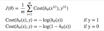
Instead of Mean Squared Error, we use a cost function called Cross-entropy loss can be divided into two separate cost functions: one for \(y=1\) and one for \(y=0\).
image
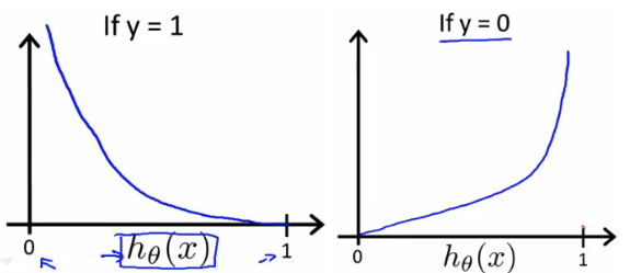
The benefits of taking the logarithm reveal themselves when you look at the cost function graphs for y=1 and y=0. These smooth monotonic functions [^2] (always increasing or always decreasing) make it easy to calculate the gradient and minimize cost. Image from Andrew Ng’s slides on logistic regression [^3].
image
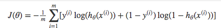
Above functions compressed into one
image
Multiplying by \(y\) and \((1-y)\) in the above equation is a sneaky trick that let’s us use the same equation to solve for both y=1 and y=0 cases. If y=0, the first side cancels out. If y=1, the second side cancels out. In both cases we only perform the operation we need to perform.
Vectorized cost function
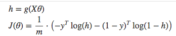
image
Code
costFunction  <- function(X, y) {

  #COSTFUNCTION Compute cost for logistic regression
  #   J <- COSTFUNCTION(theta, X, y) computes the cost of using theta as the
  #   parameter for logistic regression.

  function(theta) {
    # Initialize some useful values
    m <- length(y) # number of training examples

    # You need to return the following variable correctly
    J <- 0


    h <- sigmoid(X %*% theta)
    J <- (t(-y) %*% log(h) - t(1 - y) %*% log(1 - h)) / m
    J
    # ----------------------------------------------------
  }
}
Gradient descent
Remember that the general form of gradient descent is:
\[\begin{align*}& Repeat \; \lbrace \newline & \; \theta_j := \theta_j - \alpha \dfrac{\partial}{\partial \theta_j}J(\theta) \newline & \rbrace\end{align*}\]
We can do the derivative using calculus to get:
\[\begin{align*} & Repeat \; \lbrace \newline & \; \theta_j := \theta_j - \frac{\alpha}{m} \sum_{i=1}^m (h_\theta(x^{(i)}) - y^{(i)}) x_j^{(i)} \newline & \rbrace \end{align*}\]
A vectorized implementation is:
\[\begin{align*} \newline & \; \theta := \theta - \frac{\alpha}{m} {X^T (g(X\theta}) - y^ \rightarrow )\end{align*}\]
grad <- function(X, y) {
  #COSTFUNCTION Compute gradient for logistic regression
    #   J <- COSTFUNCTION(theta, X, y) computes the gradient of the cost
    #   w.r.t. to the parameters.
  function(theta) {

    # You need to return the following variable correctly
    grad <- matrix(0,dim(as.matrix(theta)))
    m <- length(y)

    h <- sigmoid(X %*% theta)

    # calculate grads

    grad <- (t(X) %*% (h - y)) / m

    grad
    # ----------------------------------------------------

  }
}
Pseudocode
Repeat {

  1. Calculate gradient average
  2. Multiply by learning rate
  3. Subtract from weights

}
Cost history
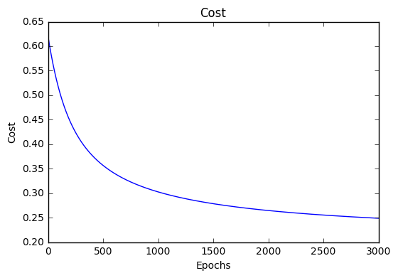
image
Accuracy
Accuracy measures how correct our predictions were. In this case we simply compare predicted labels to true labels and divide by the total.
Decision boundary
Another helpful technique is to plot the decision boundary on top of our predictions to see how our labels compare to the actual labels. This involves plotting our predicted probabilities and coloring them with their true labels.
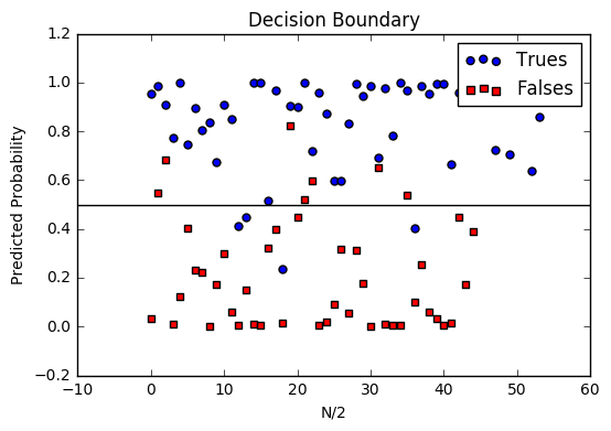
image
Multiclass logistic regression
Instead of \(y = {0,1}\) we will expand our definition so that \(y = {0,1...n}\). Basically we re-run binary classification multiple times, once for each class.
Procedure
- Divide the problem into n+1 binary classification problems (+1 because the index starts at 0?).
- For each class…
- Predict the probability the observations are in that single class.
- prediction = <math>max(probability of the classes)
For each sub-problem, we select one class (YES) and lump all the others into a second class (NO). Then we take the class with the highest predicted value.
Since y = {0,1…n}, we divide our problem into n+1 (+1 because the index starts at 0) binary classification problems; in each one, we predict the probability that ‘y’ is a member of one of our classes.
\[\begin{align*}& y \in \lbrace0, 1 ... n\rbrace \newline& h_\theta^{(0)}(x) = P(y = 0 | x ; \theta) \newline& h_\theta^{(1)}(x) = P(y = 1 | x ; \theta) \newline& \cdots \newline& h_\theta^{(n)}(x) = P(y = n | x ; \theta) \newline& \mathrm{prediction} = \max_i( h_\theta ^{(i)}(x) )\newline\end{align*}\]
Slide show
knitr::include_url('/slides/LogisticRegression.html')