Exploring and preparing data
Exploring and preparing data with titanic dataset

.badCode {
background-color: black;
}
Introduction
The first a part of any data analysis or predictive modeling task is an initial exploration of the datasets. Albeit we collected the datasets ourself and we have already got an inventory of questions in mind that we simply want to answer, it’s important to explore the datasets before doing any serious analysis, since oddities within the datasets can cause bugs and muddle your results. Before exploring deeper questions, we got to answer many simpler ones about the shape and quality of datasets . That said, it’s important to travel into initial data exploration with an enormous picture question in mind.
This post aims to boost a number of the questions we ought to consider once we check out a replacement data set for the primary time and show the way to perform various Python operations associated with those questions.
In this post, we’ll explore the Titanic disaster training set available from Kaggle.co. The dataset consists of 889 passengers who rode aboard the Titanic.
Getting the dataset
To get the dataset into pandas dataframe simply call the function read_csv.
import pandas as pd
import numpy as np

tit_train = pd.read_csv("../data/titanic/train.csv")      # Read the data
Checking the dimensions of the dataset with df.shape and the variable data types of df.dtypes.
tit_train.shape## (891, 12)tit_train.dtypes## PassengerId int64
## Survived int64
## Pclass int64
## Name object
## Sex object
## Age float64
## SibSp int64
## Parch int64
## Ticket object
## Fare float64
## Cabin object
## Embarked object
## dtype: objectThe output displays that we re working with a set of 891 records and 12 columns. Most of the column variables are encoded as numeric data types (ints and floats) but a some of them are encoded as “object”.
Check the head of the data to get a better sense of what the variables look like:
tit_train.head(5)## PassengerId Survived Pclass ... Fare Cabin Embarked
## 0 1 0 3 ... 7.2500 NaN S
## 1 2 1 1 ... 71.2833 C85 C
## 2 3 1 3 ... 7.9250 NaN S
## 3 4 1 1 ... 53.1000 C123 S
## 4 5 0 3 ... 8.0500 NaN S
##
## [5 rows x 12 columns]We have a combination of numeric columns and columns with text data.
In dataset analysis, variables or features that split records into a fixed number of unique categories, such as Sex, are called as categorical variables.
Pandas can be used to interpret categorical variables as such when we load dataset, but we can convert a variable to categorical if necessary
After getting a sense of the datasets structure, it is a good practice to look at a statistical summary of the features with df.describe():
tit_train.describe().transpose()## count mean std ... 50% 75% max
## PassengerId 891.0 446.000000 257.353842 ... 446.0000 668.5 891.0000
## Survived 891.0 0.383838 0.486592 ... 0.0000 1.0 1.0000
## Pclass 891.0 2.308642 0.836071 ... 3.0000 3.0 3.0000
## Age 714.0 29.699118 14.526497 ... 28.0000 38.0 80.0000
## SibSp 891.0 0.523008 1.102743 ... 0.0000 1.0 8.0000
## Parch 891.0 0.381594 0.806057 ... 0.0000 0.0 6.0000
## Fare 891.0 32.204208 49.693429 ... 14.4542 31.0 512.3292
##
## [7 rows x 8 columns]we notice that the non-numeric columns are omitted from the statistical summary provided by df.describe().
We can find the summary of the categorical variables by passing only those columns to describe():
cat_vars = tit_train.dtypes[tit_train.dtypes == "object"].index

print(cat_vars)
## Index(['Name', 'Sex', 'Ticket', 'Cabin', 'Embarked'], dtype='object')tit_train[cat_vars].describe().transpose()## count unique top freq
## Name 891 891 Oreskovic, Mr. Luka 1
## Sex 891 2 male 577
## Ticket 891 681 1601 7
## Cabin 204 147 C23 C25 C27 4
## Embarked 889 3 S 644The summary of the categorical features shows the count of non-NaN records, the number of unique categories, the most frequent occurring value and the number of occurrences of the most frequent value.
Although describe() gives a concise overview of each variable, it does not necessarily give us enough information to determine what each variable means.
Certain features like “Age” and “Fare” are easy to understand, while others like “SibSp” and “Parch” are not. The details of these are provided by kaggle on the data download page.
# VARIABLE DESCRIPTIONS:
# survival        Survival
#                 (0 = No; 1 = Yes)
# pclass          Passenger Class
#                 (1 = 1st; 2 = 2nd; 3 = 3rd)
# name            Name
# sex             Sex
# age             Age
# sibsp           Number of Siblings/Spouses Aboard
# parch           Number of Parents/Children Aboard
# ticket          Ticket Number
# fare            Passenger Fare
# cabin           Cabin
# embarked        Port of Embarkation
#                 (C = Cherbourg; Q = Queenstown; S = Southampton)
After looking at the data we ask yourself a few questions:
| QUESTIONS |
|---|
| Do we require all of the variables ? |
| Should we transform any variables ? |
| Check if there are any NA values, outliers etc ? |
| Should we create new variables? |
Do we require all of the Variables?
Removal of unnecessary variables is a first step when dealing with any data set, since removing variables reduces complexity and can make computation on the data faster.
Whether we should get rid of a variable or not will depend on size of the data set and the goal of the analysis. With a dataset like the titanic data, there’s no requirement to remove variables from a computing perspective. But it can be helpful to drop variables that will only distract from your goal.
Let’s go through each variable and consider whether we should keep it or not in the context of survival prediction.
“PassengerId” is just a number assigned to each passenger. We can remove it
del tit_train['PassengerId']Variable “Survived” shows whether each passenger lived or died. Since survival prediction is our goal, we definitely need to keep it.
Features describing passengers numerically or grouping them into a few broad categories could be useful for survival prediction. Therefore variables Pclass, Sex, Age, SibSp, Parch, Fare and Embarked can be kept.
further, “Name” appears to be a character string of the name of each passenger and it will also help in identifying passenger so we can keep it
Next, let’s see at “Ticket”
tit_train['Ticket'][0:10]## 0 A/5 21171
## 1 PC 17599
## 2 STON/O2. 3101282
## 3 113803
## 4 373450
## 5 330877
## 6 17463
## 7 349909
## 8 347742
## 9 237736
## Name: Ticket, dtype: objecttit_train['Ticket'].describe()## count 891
## unique 681
## top 1601
## freq 7
## Name: Ticket, dtype: objectTicket has 681 unique values: almost as many as there are passengers. Categorical variables with this many levels are generally not very useful for prediction. Let’s remove it
del tit_train['Ticket']Lastly let’s see the “Cabin” variable
tit_train['Cabin'][0:10]## 0 NaN
## 1 C85
## 2 NaN
## 3 C123
## 4 NaN
## 5 NaN
## 6 E46
## 7 NaN
## 8 NaN
## 9 NaN
## Name: Cabin, dtype: objecttit_train['Cabin'].describe()## count 204
## unique 147
## top C23 C25 C27
## freq 4
## Name: Cabin, dtype: objectCabin also has 147 unique values, which shows it may not be useful for prediction. On the other hand, the names of the different levels for the cabin variable seem to have a some structure, each starts with a capital letter followed by a number. We can use that structure to reduce the number of levels to make categories large enough that they might be useful for prediction later on. So Lets Keep Cabin for now.
Should we transform Any Variables?
Pclass is an integer variable that indicates a passenger’s class, with 1 being first class, 2 as second class and 3 as third class. We can transform this by transforming Pclass into an ordered categorical variable
pclass_new = pd.Categorical(tit_train['Pclass'], ordered=True)

pclass_new = pclass_new.rename_categories(["class1","class2","class3"])

pclass_new.describe()
## counts freqs
## categories
## class1 216 0.242424
## class2 184 0.206510
## class3 491 0.551066tit_train['Pclass'] = pclass_newNow see the Cabin variable. It appears that each Cabin is in a general section of the ship indicated by the capital letter at the start of each factor level
tit_train['Cabin'].unique()## array([nan, 'C85', 'C123', 'E46', 'G6', 'C103', 'D56', 'A6',
## 'C23 C25 C27', 'B78', 'D33', 'B30', 'C52', 'B28', 'C83', 'F33',
## 'F G73', 'E31', 'A5', 'D10 D12', 'D26', 'C110', 'B58 B60', 'E101',
## 'F E69', 'D47', 'B86', 'F2', 'C2', 'E33', 'B19', 'A7', 'C49', 'F4',
## 'A32', 'B4', 'B80', 'A31', 'D36', 'D15', 'C93', 'C78', 'D35',
## 'C87', 'B77', 'E67', 'B94', 'C125', 'C99', 'C118', 'D7', 'A19',
## 'B49', 'D', 'C22 C26', 'C106', 'C65', 'E36', 'C54',
## 'B57 B59 B63 B66', 'C7', 'E34', 'C32', 'B18', 'C124', 'C91', 'E40',
## 'T', 'C128', 'D37', 'B35', 'E50', 'C82', 'B96 B98', 'E10', 'E44',
## 'A34', 'C104', 'C111', 'C92', 'E38', 'D21', 'E12', 'E63', 'A14',
## 'B37', 'C30', 'D20', 'B79', 'E25', 'D46', 'B73', 'C95', 'B38',
## 'B39', 'B22', 'C86', 'C70', 'A16', 'C101', 'C68', 'A10', 'E68',
## 'B41', 'A20', 'D19', 'D50', 'D9', 'A23', 'B50', 'A26', 'D48',
## 'E58', 'C126', 'B71', 'B51 B53 B55', 'D49', 'B5', 'B20', 'F G63',
## 'C62 C64', 'E24', 'C90', 'C45', 'E8', 'B101', 'D45', 'C46', 'D30',
## 'E121', 'D11', 'E77', 'F38', 'B3', 'D6', 'B82 B84', 'D17', 'A36',
## 'B102', 'B69', 'E49', 'C47', 'D28', 'E17', 'A24', 'C50', 'B42',
## 'C148'], dtype=object)If we grouped the cabin just by this letter, we could lesser the number of levels while getting some useful information.
chr_cabin = tit_train["Cabin"].astype(str)

n_Cabin = np.array([cabin[0] for cabin in chr_cabin])

n_Cabin = pd.Categorical(n_Cabin)

n_Cabin.describe()
## counts freqs
## categories
## A 15 0.016835
## B 47 0.052750
## C 59 0.066218
## D 33 0.037037
## E 32 0.035915
## F 13 0.014590
## G 4 0.004489
## T 1 0.001122
## n 687 0.771044The output of describe() shows we can group Cabin into broader categories, but we also discovered something interesting: 688 of the records have Cabin are “n” which is shortened from “nan”. In other words, more than 2/3 of the passengers do not have a cabin.
A missing cabin variable could be an indication that a passenger died.
We can keep the new variable cabin
tit_train["Cabin"] = n_CabinChecking to if there are null Values, Outliers or Other garbage Values?
To check the missing values we us pd.isnull() function for example
mock_vector = pd.Series([1,None,3,None,7,8])

mock_vector.isnull()
## 0 False
## 1 True
## 2 False
## 3 True
## 4 False
## 5 False
## dtype: boolIf the missing values are numeric then they can be simple deleted. If missing values are categorical then they can be treated as additional category with value as NA.
To check if there is missing age values in titanic dataset
tit_train["Age"].describe()## count 714.000000
## mean 29.699118
## std 14.526497
## min 0.420000
## 25% 20.125000
## 50% 28.000000
## 75% 38.000000
## max 80.000000
## Name: Age, dtype: float64We see that the count of age (712) is less than the total row count of dataset(889).
To check indexes of the missing ages we use np.where()
missvalues = np.where(tit_train["Age"].isnull() == True)
missvalues
## (array([ 5, 17, 19, 26, 28, 29, 31, 32, 36, 42, 45, 46, 47,
## 48, 55, 64, 65, 76, 77, 82, 87, 95, 101, 107, 109, 121,
## 126, 128, 140, 154, 158, 159, 166, 168, 176, 180, 181, 185, 186,
## 196, 198, 201, 214, 223, 229, 235, 240, 241, 250, 256, 260, 264,
## 270, 274, 277, 284, 295, 298, 300, 301, 303, 304, 306, 324, 330,
## 334, 335, 347, 351, 354, 358, 359, 364, 367, 368, 375, 384, 388,
## 409, 410, 411, 413, 415, 420, 425, 428, 431, 444, 451, 454, 457,
## 459, 464, 466, 468, 470, 475, 481, 485, 490, 495, 497, 502, 507,
## 511, 517, 522, 524, 527, 531, 533, 538, 547, 552, 557, 560, 563,
## 564, 568, 573, 578, 584, 589, 593, 596, 598, 601, 602, 611, 612,
## 613, 629, 633, 639, 643, 648, 650, 653, 656, 667, 669, 674, 680,
## 692, 697, 709, 711, 718, 727, 732, 738, 739, 740, 760, 766, 768,
## 773, 776, 778, 783, 790, 792, 793, 815, 825, 826, 828, 832, 837,
## 839, 846, 849, 859, 863, 868, 878, 888], dtype=int64),)len(missvalues)## 1Before we do anything with missing values its good to check the distribution of the missing values to know the central tendency of age.
tit_train.hist(column='Age',
                   figsize=(9,6),
bins=20) 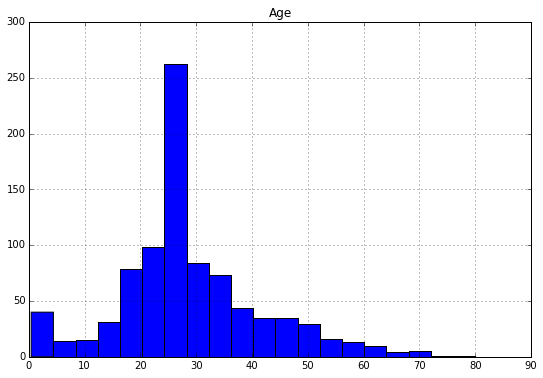
The histogram shows that couple of passengers are near age 80.
To check the fare variable we create the box plot
tit_train["Fare"].plot(kind="box",
                           figsize=(9,9))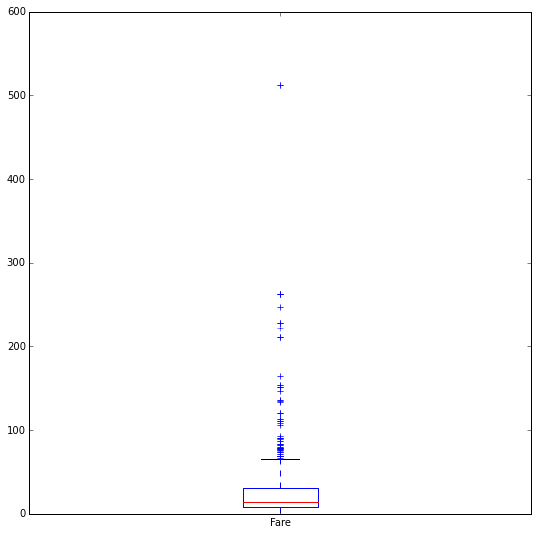
50% of the data in the box plot represents the median. There are outliers in the data. There are passengers who paid double the amount than any other passenger. We can check this using np.where() function
ind = np.where(tit_train["Fare"] == max(tit_train["Fare"]) )

tit_train.loc[ind]
## Survived Pclass ... Cabin Embarked
## 258 1 class1 ... n C
## 679 1 class1 ... B C
## 737 1 class1 ... B C
##
## [3 rows x 10 columns]Before modeling datasets using ML models it is better to address missing values, outliers, mislabeled data, bad data because they can corrupt the analysis and lead to wrong results.
Should we Create New Variables?
The decision to create new variables should be taken while preparing the data. The new variable could represent aggregate of existing variables, for example in titanic dataset we can create a new variable called family which stores the number of members in that family.
tit_train["Family"] = tit_train["SibSp"] + tit_train["Parch"]we can check who has most family members on the board
mostfamily = np.where(tit_train["Family"] == max(tit_train["Family"]))

tit_train.loc[mostfamily]
## Survived Pclass Name ... Cabin Embarked Family
## 159 0 class3 Sage, Master. Thomas Henry ... n S 10
## 180 0 class3 Sage, Miss. Constance Gladys ... n S 10
## 201 0 class3 Sage, Mr. Frederick ... n S 10
## 324 0 class3 Sage, Mr. George John Jr ... n S 10
## 792 0 class3 Sage, Miss. Stella Anna ... n S 10
## 846 0 class3 Sage, Mr. Douglas Bullen ... n S 10
## 863 0 class3 Sage, Miss. Dorothy Edith "Dolly" ... n S 10
##
## [7 rows x 11 columns]Summary
There are question that should be answered while investing any dataset. Once the basic questions are answered one can move further to find relationship between variables/features and build the machine learning models.