Getting the dataset

To get the dataset into pandas dataframe simply call the function read_csv.

import pandas as pd
import numpy as np
mt_car = pd.read_csv("../data/mtcars/mt_car.csv")      # Read the data

Center and Scale

To center and scale the dataset we substract the mean value from each data point. Subtracting the mean centers the data around zero and sets the new mean to zero. Lets try do it with mtcars dataset.

print (mt_car.head() )

##    m_pg  n_cyl  disp_ment   n_hp   dra   w_t  q_sec  v_s  a_m  n_gear  n_carb
## 0  21.0    6.0      160.0  110.0  3.90  2.62  16.46  0.0  1.0     4.0     4.0
## 1  21.0    6.0      160.0  110.0  3.90  2.88  17.02  0.0  1.0     4.0     4.0
## 2  22.8    4.0      108.0   93.0  3.85  2.32  18.61  1.0  1.0     4.0     1.0
## 3  21.4    6.0      258.0  110.0  3.08  3.22  19.44  1.0  0.0     3.0     1.0
## 4  18.7    8.0      360.0  175.0  3.15  3.44  17.02  0.0  0.0     3.0     2.0

col_means = mt_car.sum()/mt_car.shape[0]  # Get column means

col_means

## m_pg          20.090625
## n_cyl          6.187500
## disp_ment    230.721875
## n_hp         146.687500
## dra            3.596563
## w_t            3.218437
## q_sec         17.848750
## v_s            0.437500
## a_m            0.406250
## n_gear         3.687500
## n_carb         2.812500
## dtype: float64

Now we need to subtract the means of the column from each row in element-wise way to zero center the data. Pandas can peform math operations involving dataframews and columns on element-wise row-by-row basis by default so it can be simply subtracted from column means series from the dataset to center it.

center_ed = mt_car - col_means

print(center_ed.describe())

##                m_pg      n_cyl     disp_ment  ...        a_m     n_gear   n_carb
## count  3.200000e+01  32.000000  3.200000e+01  ...  32.000000  32.000000  32.0000
## mean   3.996803e-15   0.000000 -4.618528e-14  ...   0.000000   0.000000   0.0000
## std    6.026948e+00   1.785922  1.239387e+02  ...   0.498991   0.737804   1.6152
## min   -9.690625e+00  -2.187500 -1.596219e+02  ...  -0.406250  -0.687500  -1.8125
## 25%   -4.665625e+00  -2.187500 -1.098969e+02  ...  -0.406250  -0.687500  -0.8125
## 50%   -8.906250e-01  -0.187500 -3.442188e+01  ...  -0.406250   0.312500  -0.8125
## 75%    2.709375e+00   1.812500  9.527812e+01  ...   0.593750   0.312500   1.1875
## max    1.380938e+01   1.812500  2.412781e+02  ...   0.593750   1.312500   5.1875
## 
## [8 rows x 11 columns]

After centering the data we see that negative values are below average while positive values are above average. Next we can put it on common scale using the standard deviation as.

col_deviations = mt_car.std(axis=0)   # Get column standard deviations

center_n_scale = center_ed/col_deviations 

print(center_n_scale.describe())

##                m_pg         n_cyl  ...        n_gear        n_carb
## count  3.200000e+01  3.200000e+01  ...  3.200000e+01  3.200000e+01
## mean   6.661338e-16 -2.775558e-17  ... -2.775558e-17  2.775558e-17
## std    1.000000e+00  1.000000e+00  ...  1.000000e+00  1.000000e+00
## min   -1.607883e+00 -1.224858e+00  ... -9.318192e-01 -1.122152e+00
## 25%   -7.741273e-01 -1.224858e+00  ... -9.318192e-01 -5.030337e-01
## 50%   -1.477738e-01 -1.049878e-01  ...  4.235542e-01 -5.030337e-01
## 75%    4.495434e-01  1.014882e+00  ...  4.235542e-01  7.352031e-01
## max    2.291272e+00  1.014882e+00  ...  1.778928e+00  3.211677e+00
## 
## [8 rows x 11 columns]

We see that after dividing by the standard deviation, every variable now has a standard deviation of 1. At this point, all the columns have roughly the same mean and scale of spread about the mean.

Manually centering and scaling is a good exercise, but it is often possible to perform common data preprocessing using functions available in the Python libraries. The Python library scikit-learn, a package for predictive modeling and data analysis, has pre-processing tools including a scale() function for centering and scaling data:

from sklearn import preprocessing

scale_data = preprocessing.scale(mt_car)  
 
scale_car = pd.DataFrame(scale_data, index = mt_car.index,
                           columns=mt_car.columns)

print(scale_car.describe() )

##                m_pg         n_cyl  ...        n_gear        n_carb
## count  3.200000e+01  3.200000e+01  ...  3.200000e+01  3.200000e+01
## mean  -4.996004e-16  2.775558e-17  ... -2.775558e-17 -2.775558e-17
## std    1.016001e+00  1.016001e+00  ...  1.016001e+00  1.016001e+00
## min   -1.633610e+00 -1.244457e+00  ... -9.467293e-01 -1.140108e+00
## 25%   -7.865141e-01 -1.244457e+00  ... -9.467293e-01 -5.110827e-01
## 50%   -1.501383e-01 -1.066677e-01  ...  4.303315e-01 -5.110827e-01
## 75%    4.567366e-01  1.031121e+00  ...  4.303315e-01  7.469671e-01
## max    2.327934e+00  1.031121e+00  ...  1.807392e+00  3.263067e+00
## 
## [8 rows x 11 columns]

preprocessing.scale() returns ndarrays which needs to be converted back to dataframe.

Handling Skewed-data

To understand whether the data is skewed or not we need to plot it. The overall shape and how the data is spread out can have a significant impact on the analysis and modeling

norm_dist = np.random.normal(size=10000) 
norm_dist= pd.DataFrame(norm_dist)
norm_dist.hist(figsize=(8,8), bins=30)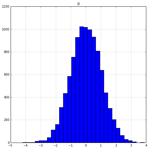

Notice how the normally distributed data looks roughly symmetric with a bell-shaped curve. Now let’s generate some skewed data

skew = np.random.exponential(scale=2, size= 10000) 
skew = pd.DataFrame(skew)
skew.hist(figsize=(8,8),bins=50)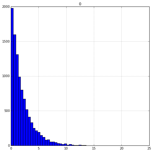

Correlation

The model that we use in predictive modeling have features and each feature is related to other features in some way or the other. Using corr() we can find how these features are related with each other