K nearest Neighbours
K nearest Neighbours

K nearest Neighbours
If there are several groups of labeled samples and the items present in the groups are homogeneous in nature. Now, assume that we have an unlabeled example which needs to be classified into one of those several labeled groups. How do we do that? Using kNN Algorithm. k nearest neighbors is an algorithm that knows all the available cases and classify the new cases by a majority vote of its k neighbors. This algorithms segregates unlabeled data points into well defined groups. KNN classifies a categorical value using the majority votes of nearest neighbors.
Input/Output/parameter
The input to a KNN classifier can be both quantitative and qualitative. The output from a KNN classifer are categorical values which typically are the class of the data.
Distance metric
A distance metric is used to define proximity between ant two data points. The examples are Euclidean distance, Manhattan distance or Hamming distance.
The Euclidean distance is used to be applied to categorical data.
Manhattan distance is used over the Euclidean distance when there is high dimensionality in the data. Manhattan distance (or block distance) is appropriate when we have a discrete data set and the Euclidean distance is appropriate when we have continuous numerical variables.
Both Euclidean and Manhattan distances are used in case of discrete/continuous variables, whereas hamming distance is used in case of categorical variable.
Example
Let us assume that we have a blind tasting experience, in which we need to classify what food we tasted as fruit, protein, or vegetable. Suppose that prior to eating the mystery item, we created a taste dataset in which we recorded two features of each ingredient: A measure from 1 to 10 on how crunchy the food is and second a score from 1 to 10 of how sweet the ingredient tastes. Then we labeled each ingredient as one of the three types of food: fruits,vegetables or proteins. We could have a table such as:
import pandas as pd
ingredient = ['apple', 'bacon', 'banana', 'carrot', 'celery', 'cheese','grape','green bean','nuts','orange']
sweetness = [10,1,10,7,3,1,8,3,3,7]
crunchiness = [9,4,1,10,10,1,5,7,6,3]
food_type = ['fruit','protein','fruit','vegetable','vegetable','protein','fruit','vegetable','protein','fruit']
df = pd.DataFrame(list(zip(ingredient,sweetness,crunchiness,food_type)), columns =['ingredient', 'sweetness','crunchiness','food_type'])
print(df)
## ingredient sweetness crunchiness food_type
## 0 apple 10 9 fruit
## 1 bacon 1 4 protein
## 2 banana 10 1 fruit
## 3 carrot 7 10 vegetable
## 4 celery 3 10 vegetable
## 5 cheese 1 1 protein
## 6 grape 8 5 fruit
## 7 green bean 3 7 vegetable
## 8 nuts 3 6 protein
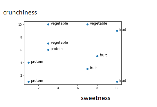
## 9 orange 7 3 fruitThe kNN algorithm treats the features as coordinates in a multidimensional feature space. As our dataset includes only two features, the feature space is 2 dimensional, with the x dimension indicating the ingredient sweetness and the y dimension indicating the crunchiness.
import matplotlib.pyplot as plt
x = sweetness
y = crunchiness
labs = food_type
plt.scatter(x, y)
for i, txt in enumerate(labs):
    plt.annotate(txt, (x[i]+.25, y[i]), fontsize=12)
Similar types of food tend to be grouped closely together.As illustrated in the next figure, vegetables tend to be crunchy but not sweet, fruits tend to be sweet and either crunchy or not crunchy, while proteins tend to be neither crunchy nor sweet
Suppose that after constructing this dataset we need to find if tomato a fruit or a vegetable. We can use a nearest neighbor approach to determine which class is a better fit as shown in the following figure:
Calculating distance:
Locating an object nearest neighbors requires a distance function or a formula that will measure the similarity between two instances. Traditionally the kNN algorithm uses the Euclidian distance. Euclidian distance is specified by the following formula, where p and q are instances to be compared, each having n features
The term p1 refers to the value of the first feature in p, while q1 refers to the first feature of q.
\[dist (p, q) = √(𝑝1 − 𝑞1)^2 + (𝑝2 − 𝑞2)^2 + ⋯ (𝑝^ n − 𝑞^𝑛)\]
The distance formula involves comparing the values of each feature. For example, to calculate the distance between the tomato (sweetness = 6, crunchiness = 4), and the green bean (sweetness = 3, crunchiness = 7), we can use the formula as follows:
\[dist(tomato, green bean) = \sqrt(6-3)^2 + (4−7)^2 = 4.2\]
In a similar vein, we can calculate the distance between the tomato and several of its closest neighbors as follows:
| ingradient | sweetness | crunchness | food type | distanct to the tomato |
|---|---|---|---|---|
| grape | 8 | 5 | fruit | \[\sqrt((6 - 8)^2 + (4 - 5)^2) = 2.2 \] |
| green bean | 3 | 7 | vegetable | \[\sqrt((6 - 3)^2 + (4 - 7)^2) = 4.2 \] |
| nuts | 3 | 6 | protein | \[\sqrt((6 - 3)^2 + (4 - 6)^2) = 3.6 \] |
| orange | 7 | 3 | fruit | \[\sqrt((6 - 7)^2 + (4 - 3)^2) = 1.4 \] |
To classify the tomato as vegetable, fruit or protein, we’ll begin by assigning the tomato the food type of its single nearest neighbor. This is called 1NN because k =1. The orange is the nearest neighbor to the tomato, with a distance of 1.4. As orange is a fruit, the 1NN algorithm would classify tomato as a fruit. If we use the kNN algorithm with k=3 instead, it performs a vote among the three nearest neighbors: orange, grape, and nuts.
Applying KNNClassifier:
The features list consists of the sweetness and crunchiness values. The target which is a categorical value is encoded using LabelEncoder.
from sklearn.preprocessing import LabelEncoder as le
features = list(zip (sweetness, crunchiness))
food_type = ['fruit','protein','fruit','vegetable','vegetable','protein','fruit','vegetable','protein','fruit']
target = le.fit_transform(food_type)
target_lables = food_type
target_df = pd.DataFrame(food_type,target)
target_df
0:fruit, 1:protein, 2:vegetable
KNeighborsClassifier created with neighbors = 2. Inside the model we fit the data with the features and encoded target
model = KNeighborsClassifier(n_neighbors=2)
model.fit(features,target)
After that we using the model we predict the food_type for new data (‘Orange’,sweetness = 6, crunchines = 4)
predicted= model.predict([[6,4]])
print(predicted)
[0]
The predicted class 0 belongs to the food type of ‘fruit’.
Choosing an appropriate k
Deciding how many neighbrs to be used for kNN determines how well the model will generalize to future data. The balance between overfitting or underfitting the training data is a problem called as the bias/variance tradeoff. Choosing greater k reduce the variance caused by noisy data, but it can bias the learner and can run the risk of ignoring small but important patterns.
Smaller k values cause complex decision boundaries that more carefully fit the training data and can overfit.
In practice, choosing k-value depends on the complexity of the concept to be learned and the number of records in the training data.
Generally, k is set between 3 and 10. One common practice is setting the k equal to the square root of the number of training example.
In the food classifier, we can set it to 4 assuming that there are 15 examples in the training data set. An alternative value is to test multiple values of k on different test datasets and select the one that delivers the best classification performance.
In the example above because the majority class among these neighbors is fruit (2 out of 3 votes), the tomato again is classified as a fruit.
Algorithm
The KNN classification is performed using the following four steps
Compute the distance metric between the test data point and all the labeled data points
Order the labeled data points in the increasing order of this distance metric
Select the top k labeled data points and look at the class labels
Find the class label that the majority of these k labeled data points have and assign it to the test data point.
There are various things like Parameter selection, Presence of noise, Feature selection and scaling, Curse of dimensionality we need to consider before applying KNN algorithm
K fold cross validation
In order to evaluate the performance of KNN classifier there are different approaches. One approach is separating the data have into a training and test set. but it can be difficult to decide what the ratio should be between the sets. Outliers and other factor will greatly influence the results of how the classifier is built and the reported accuracy.
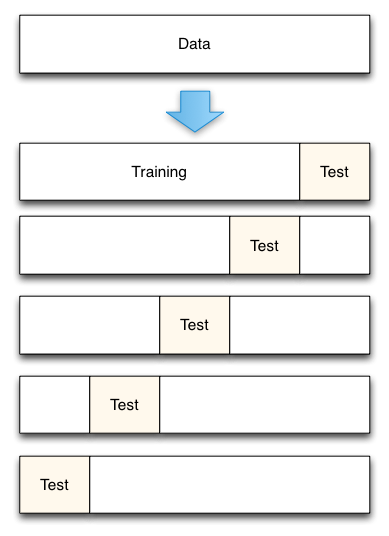
Another approach is called as k-fold cross validation. In this approach, the data is divided up in to k equally sized pieces. One of these pieces is saved for test data and the remaining k − 1 pieces are used for training. We then buiid the model k times, rotating the piece we use for testing. We can judge the performance of the classifier on its average accuracy and standard dev.
k fold example
Split the dataset into K equal partitions (or “folds”) therefore if k = 4 and dataset has 120 observations then each of the 4 folds will have 30 observations. After that make use of the fold 1 as the testing set and the union of the other folds as the training set. Therefore in this case we will have testing set = 30 observations (fold 1), Training set = 90 observations (folds 2-4). After that calculate the testing accuracy. There after by repeating above steps K times, using a different fold as the testing set each time. We will need to repeat the process 4 times. In 2nd iteration fold 2 will be testing set and union of 1,3,4 will be training set and so on..Finally use the mean testing accuracy as the estimate of out-of-sample accuracy.

# simulate splitting a dataset of 25 observations into 5 folds
from sklearn.model_selection import KFold
import numpy as np
kf = KFold(n_splits=5, random_state=None, shuffle=False)
Vec = np.arange(0,25)
# print the contents of each training and testing set
print('{} {:^61} {}'.format('Iteration',
                            'Training set observations',
                            'Testing set observations'))
## Iteration Training set observations Testing set observationsfor iteration, data in enumerate(kf.split(Vec), start=1):
print('{:^9} {} {!s:^25}'.format(iteration, data[0], data[1]))## 1 [ 5 6 7 8 9 10 11 12 13 14 15 16 17 18 19 20 21 22 23 24] [0 1 2 3 4]
## 2 [ 0 1 2 3 4 10 11 12 13 14 15 16 17 18 19 20 21 22 23 24] [5 6 7 8 9]
## 3 [ 0 1 2 3 4 5 6 7 8 9 15 16 17 18 19 20 21 22 23 24] [10 11 12 13 14]
## 4 [ 0 1 2 3 4 5 6 7 8 9 10 11 12 13 14 20 21 22 23 24] [15 16 17 18 19]
## 5 [ 0 1 2 3 4 5 6 7 8 9 10 11 12 13 14 15 16 17 18 19] [20 21 22 23 24]

