Support Vector Machines

Support Vector Machines are very powerful, very efficient machine learning algorithms and they even achieve much better results than neural networks in some areas. We are again dealing with classification here but the methodology is quite different.

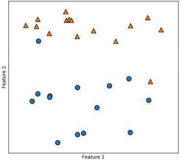
What we are looking for is a hyperplane that distinctly classifies our data points and has the maximum margin to all of our points. We want our model to be as generalized as possible.

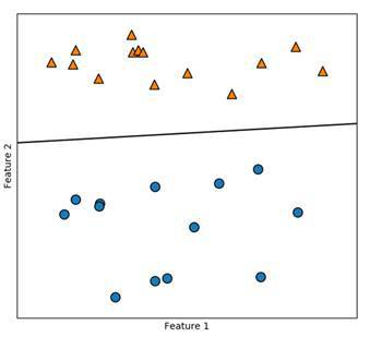
In the graph above the model is very general and the line is the optimal function to separate our data. We can use an endless amount of lines to separate the two classes but we don’t want to overfit our model so that it only works for the data we already have. We also want it to work for unknown data.

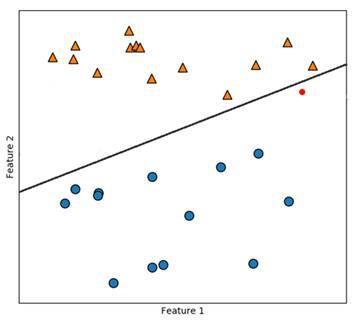
Here our model also separates the data we already have perfectly. But we’ve got a new red data point here. When we just look at this with our intuition it is obvious that this point belongs to the orange triangles. However, our model classifies it as a blue circle because it is overfitting our current data. To find our perfect line we are using so-called support vectors , which are parallel lines.

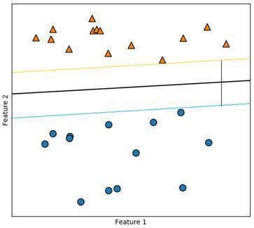
We are looking for the two points that are the farthest away from the other class. In between of those, we draw our hyperplane so that the distance to both points is the same and as large as possible. The two parallel lines are the support vectors. In between the orange and the blue line there are no data points. This is our margin. We want this margin to be as big as possible because it makes our predictions more reliable.

KERNELS

The data we have looked at so far is relatively easy to classify because it is clearly separated. Such data can almost never be found in the real world. Also, we are oftentimes working in higher dimensions with many features. This makes things more complicated.

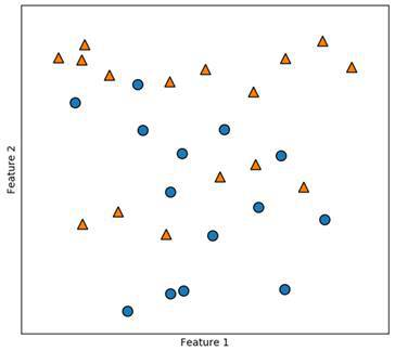
Data taken from the real world often looks like this in figure. Here it is impossible to draw a straight line, and even a quadratic or cubic function does not help us here. In such cases we can use so-called kernels . These add a new dimension to our data. By doing that, we hope to increase the complexity of the data and possibly use a hyperplane as a separator.

Notice that the kernel (a.k.a. the additional dimension) should be derived from the data that we already have. We are just making it more abstract. A kernel is not some random feature but a combination of the features we already have. But that wouldn’t be reasonable or helpful. Therefore, there are pre-defined and effective kernels that we can choose from.

SOFT MARGIN

Sometimes, we will encounter statistical outliers in our data. It would be very easy to draw a hyperplane that separates the data into the classes, if it wasn’t for these outliers.

n the figure above, you can see such a data set. We can see that almost all of the orange triangles are in the top first third, whereas almost all the blue dots are in the bottom two thirds. The problem here is with the outliers. Now instead of using a kernel or a polynomial function to solve this problem, we can define a so-called soft margin. With this, we allow for conscious misclassification of outliers in order to create a more accurate model. Caring too much about these outliers would again mean overfitting the model.

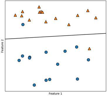As you can see, even though we are misclassifying two data points our model is very accurate.

LOADING DATA

Now that we understand how SVMs work, let’s get into the coding. For this machine learning algorithm, we are going to once again use the breast cancer data set. We will need the following imports:

from sklearn.svm import SVC
from sklearn.datasets import load_breast_cancer
from sklearn.neighbors import KNeighborsClassifier
from sklearn.model_selection import train_test_split 

Besides the libraries we already know, we are importing the SVC module. This is the support vector classifier that we are going to use as our model. Notice that we are also importing the KNeighborsClassifier again, since we are going to compare the accuracies at the end.

data = load_breast_cancer()
X = data.data
Y = data.target
X_train, X_test, Y_train, Y_test = train_test_split(X, Y, test_size = 0.1 , random_state = 30 )

This time we use a new parameter named random_state . It is a seed that always produces the exact same split of our data. Usually, the data gets split randomly every time we run the script. You can use whatever number you want here. Each number creates a certain split which doesn’t change no matter how many times we run the script. We do this in order to be able to objectively compare the different classifiers.

TRAINING AND TESTING

So first we define our support vector classifier and start training it.

model = SVC( kernel = 'linear' , C = 3 )
model.fit(X_train, Y_train)

## SVC(C=3, kernel='linear')

We are using two parameters when creating an instance of the SVC class. The first one is our kernel and the second one is C which is our soft margin. Here we choose a linear kernel and allow for three misclassifications. Alternatively we could choose poly, rbf, sigmoid, precomputed or a self-defined kernel. Some are more effective in certain situations but also a lot more time-intensive than linear kernels.

accuracy = model.score(X_test, Y_test)
print (accuracy)

## 0.9649122807017544

When we now score our model, we will see a very good result. 0.9649122807017544