Neural Network using Make Moons dataset
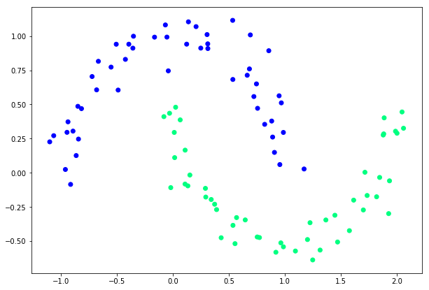
The make_moons dataset is a swirl pattern, or two moons. It is a set of points in 2D making two interleaving half circles. It displays 2 disjunctive clusters of data in a 2-dimensional representation space ( with coordinates x1 and x2 for two features). The areas are formed like 2 moon crescents as shown in the figure below.
Neural Network using Make Moons dataset
Make moons dataset
The make_moons dataset is a swirl pattern, or two moons. It is a set of points in 2D making two interleaving half circles. It displays 2 disjunctive clusters of data in a 2-dimensional representation space ( with coordinates x1 and x2 for two features). The areas are formed like 2 moon crescents as shown in the figure below.
Importing libraries
from sklearn import datasets
import numpy as np
import matplotlib.pyplot as plt
from sklearn.model_selection import train_test_split
numpy is used for scientific computing with Python. It is one of the fundamental packages you will use. Matplotlib library is used in Python for plotting graphs. The datasets package is the place from where you will import the make moons dataset. Sklearn library is used fo scientific computing. It has many features related to classification, regression and clustering algorithms including support vector machines.
Initializing the dataset
np.random.seed(0)
feature_set_x, labels_y = datasets.make_moons(100, noise=0.10)
X_train, X_test, y_train, y_test = train_test_split(feature_set_x, labels_y, test_size=0.33, random_state=42)
In the script above we import the datasets class from the sklearn library. To create non-linear dataset of 100 data-points, we use the make_moons method and pass it 100 as the first parameter. The method returns a dataset, which when plotted contains two interleaving half circles. Data cannot be separated by a single straight line, hence the perceptron cannot be used to correctly classify make moons dataset.
Build the neural network model using keras
from keras.models import Sequentialmodel = Sequential()Basically there are two types of models in Keras. Sequential and Functional.
The sequential API is generally used and helps in creating the models layer-by-layer for most problems. It is constrained in that it does not allow us to create models that share layers or have multiple inputs or outputs.
The functional API helps in creating models that have a lot more flexibility as we can easily define models where layers connect to more than just the previous and next layers. In fact, we can connect layers to any other layer. As a result, creating complex networks become possible.
from keras.layers import Dense, ActivationA dense layer is a Layer in which Each Input Neuron is connected to the output Neuron, like a Simple neural net, the parameters units just tells you the dimensionnality of your Output.
model.add(Dense(50, input_dim=2, activation='relu'))
model.add(Dense(1, activation='sigmoid'))
Sample neural network using two hidden layers
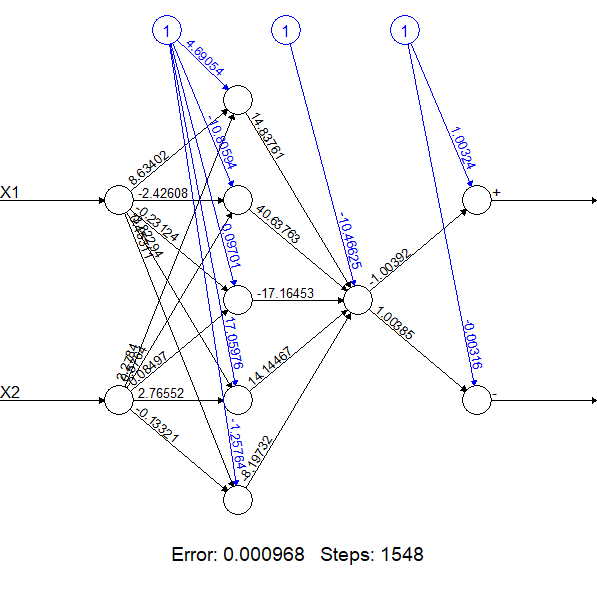
For example if you say Dense(50, input_dim = 2..) this means that input neurons having dimension of 2 i.e 2 input neurons are connected to dense layer having 50 neurons and at each of the neuron in dense layer is applying activation function as relu for computing the output of that neuron. These 50 neurons in the hidden layer are then connected to one neuron in the output layer with activation function of sigmoid.
model.compile(loss='binary_crossentropy', optimizer='adam', metrics= ['accuracy'])The output that we are trying to predict is having 2 classes therefore we are using ‘Binary Crossentropy’ loss function. Adam is a replacement optimization algorithm for stochastic gradient descent for training deep learning models. Adam combines the best properties of the AdaGrad and RMSProp algorithms to provide an optimization algorithm that can handle sparse gradients on noisy problems.
print(model.summary())## Model: "sequential_1"
## _________________________________________________________________
## Layer (type) Output Shape Param #
## =================================================================
## dense_1 (Dense) (None, 50) 150
## _________________________________________________________________
## dense_2 (Dense) (None, 1) 51
## =================================================================
## Total params: 201
## Trainable params: 201
## Non-trainable params: 0
## _________________________________________________________________
## NoneThe model summary gives the number of parameters input to the model. Theare are total 201 parameters including the parameters from the bias unit. The two input units and one bias unit are fed via connection links to 50 neurons totaling 150 parameters, there after the hidden layer is connected to the 1 output and 1 bias unit also is connected to output neuron. Thus the computation of the paraters will be 150(Input, bias unit to hidden layer with 50 neurons) + 50(hidden layer to output) + 1 (bias unit in the output) = 201.
Train and evaluate the model
results = model.fit(X_train, y_train , nb_epoch=100)Once the model is compiled then we use the training data to train the model via the fit function having parameters such as features set and the target label and number of iterations. Once the training is complete we evaluate the model to determine the loss and the accuracy.
score = model.evaluate(X_test, y_test, verbose=0)
print('Test score:', score[0])
## Test score: 0.3024758290160786print('Test accuracy:', score[1])## Test accuracy: 0.8787878751754761The lower the loss, the better a model (unless the model has over-fitted to the training data). The loss is calculated on training and validation and its interpretation is how well the model is doing for these two sets. Unlike accuracy, loss is not a percentage. It is a summation of the errors made for each example in training or validation sets.
The accuracy of a model is usually determined after the model parameters are learned and fixed and no learning is taking place. Then the test samples are fed to the model and the number of mistakes (zero-one loss) the model makes are recorded, after comparison to the true targets. Then the percentage of miss classification is calculated.
For example, if the number of test samples is 1000 and model classifies 875 of those correctly, then the model’s accuracy is 87.5%.
Evaluate prediction accuracy
from sklearn import metrics
prediction_values = model.predict_classes(X_test)
print(metrics.confusion_matrix(y_test, prediction_values))
## [[14 2]
## [ 2 15]]print(metrics.classification_report(y_test, prediction_values))## precision recall f1-score support
##
## 0 0.88 0.88 0.88 16
## 1 0.88 0.88 0.88 17
##
## accuracy 0.88 33
## macro avg 0.88 0.88 0.88 33
## weighted avg 0.88 0.88 0.88 33Classification report is used to evaluate a model’s predictive power. It provides Precision, Recall,F1-score,Support that will help in evaluating the model.
We can see here that on average the model has predicted 88% of the classification correctly.For Class 0 it has predicted 88% of the test data correctly.
Classification_report is also useful when comparing two models with different specifications against each other and determining which model is better to use.