Pandas (Python)
Pandas is a software module for the Python programming language for the purpose of data manipulation and analysis. It provides data structures and operations to manipulate numerical tables and time series data. It is build on top of numpy. It is applied for fast analysis and data cleaning and preparation.In this post we will learn various wasy to work with Pandas DataFrames.
Pandas
Pandas is probably the most powerful library. It provides high-performance tools for data manipulation and analysis. Furthermore, it is very effective at converting data formats and querying data out of databases. The two main data structures of Pandas are the series and the data frame. To work with Pandas, we need to import the module.
import pandas as pdPandas Series
A series in Pandas is a one-dimensional array which is labeled. You can imagine it to be the equivalent of an ordinary Python dictionary.
series = pd.Series([ 10 , 20 , 30 , 40 ],
[ 'A' , 'B' , 'C' , 'D' ])
In order to create a series, we use the constructor of the Series class. The first parameter that we pass is a list full of values (in this case numbers). The second parameter is the list of the indices or keys (in this case strings). When we now print our series, we can see what the structure looks like.
print(series)## A 10
## B 20
## C 30
## D 40
## dtype: int64The first column represents the indices, whereas the second column represents the actual values.
ACCESSING VALUES
The accessing of values works in the same way that it works with dictionaries. We need to address the respective index or key to get our desired value.
print (series[ 'C' ])## 30print (series[ 1 ])## 20As you can see, we can choose how we want to access our elements. We can either address the key or the position that the respective element is at.
CONVERTING DICTIONARIES
Since series and dictionaries are quite similar, we can easily convert our Python dictionaries into Pandas series.
myDict = { 'A' : 10 , 'B' : 20 , 'C' : 30 }
series = pd.Series(myDict)
Now the keys are our indices and the values remain values. But what we can also do is, to change the order of the indices.
myDict = { 'A' : 10 , 'B' : 20 , 'C' : 30 }
series = pd.Series(myDict, index =[ 'C' , 'A' , 'B' ])
Our series now looks like this:
print(series)## C 30
## A 10
## B 20
## dtype: int64PANDAS DataFrame
DataFrame is the main thing on which we’ll be mostly working on. Most manipulation or operation on the data will be applied by means of DataFrame.
Creating DataFrame using dictionary data
This is a simple process in which we just need to pass the json data to the DataFrame method.
cars = {'Brand':['Honda','Toyota','Ford','Audi'],'Price':[22000,21000,27000,35000]}
df = pd.DataFrame(cars)
df
## Brand Price
## 0 Honda 22000
## 1 Toyota 21000
## 2 Ford 27000
## 3 Audi 35000data = { 'Name' : [ 'Anna' , 'Bob' , 'Charles' ], 'Age' : [ 24 , 32 , 35 ], 'Height' : [ 176 , 187 , 175 ]}
df = pd.DataFrame(data)To create a Pandas data frame, we use the constructor of the class. In this case, we first create a dictionary with some data about three persons. We feed that data into our data frame. It then looks like this:
df## Name Age Height
## 0 Anna 24 176
## 1 Bob 32 187
## 2 Charles 35 175As you can see, without any manual work, we already have a structured data frame and table.
To now access the values is a bit more complicated than with series. We have multiple columns and multiple rows, so we need to address two values.
print (df[ 'Name' ][ 1 ])## BobSo first we choose the column Name and then we choose the second element (index one) of this column. In this case, this is Bob .
When we omit the last index, we can also select only the one column. This is useful when we want to save specific columns of our data frame into a new one. What we can also do in this case is to select multiple columns.
print (df[[ 'Name' , 'Height' ]])## Name Height
## 0 Anna 176
## 1 Bob 187
## 2 Charles 175DATA FRAME FUNCTIONS
For data frames we have a couple of basic functions and attributes that we already know from lists or NumPy arrays.
| BASIC FUNCTIONS AND ATTRIBUTES | |
|---|---|
| df.T | Transposes the rows and columns of the data frame |
| df.dtypes | Returns data types of the data frame |
| df.ndim | Returns the number of dimensions of the data frame |
| df.shape | Returns the shape of the data frame |
| df.size | Returns the number of elements in the data frame |
| df.head(n) | Returns the first n rows of the data frame (default is five) |
| df.tail(n) | Returns the last n rows of the data frame (default is five) |
STATISTICAL FUNCTIONS
For the statistical functions, we will now extend our data frame a little bit and add some more persons.
data = { 'Name' : [ 'Anna' , 'Bob' , 'Charles' ,
'Daniel' , 'Evan' , 'Fiona' ,
'Gerald' , 'Henry' , 'India' ],
'Age' : [ 24 , 32 , 35 , 45 , 22 , 54 , 55 , 43 , 25 ],
'Height' : [ 176 , 187 , 175 , 182 , 176 ,
189 , 165 , 187 , 167 ]}
df = pd.DataFrame(data)| STATISTICAL FUNCTIONS | |
|---|---|
| FUNCTION | DESCRIPTION |
| count() | Count the number of non-null elements |
| sum() | Returns the sum of values of the selected columns |
| mean() | Returns the arithmetic mean of values of the selected columns |
| median() | Returns the median of values of the selected columns |
| mode() | Returns the value that occurs most often in the columns selected |
| std() | Returns standard deviation of the values |
| min() | Returns the minimum value |
| max() | Returns the maximum value |
| abs() | Returns the absolute values of the elements |
| prod() | Returns the product of the selected elements |
| describe() | Returns data frame with all statistical values summarized |
Now, we are not going to dig deep into every single function here. But let’s take a look at how to apply some of them.
print (df[ 'Age' ].mean())## 37.22222222222222print (df[ 'Height' ].median())## 176.0Here we choose a column and then apply the statistical functions on it. What we get is just a single scalar with the desired value.
We can also apply the functions to the whole data frame. In this case, we get returned another data frame with the results for each column.
print (df.mean())## Age 37.222222
## Height 178.222222
## dtype: float64APPLYING NUMPY FUNCTIONS
Instead of using the built-in Pandas functions, we can also use the methods we already know. For this, we just use the apply function of the data frame and then pass our desired method.
import numpy as np
print (df[ 'Age' ].apply(np.sin))
## 0 -0.905578
## 1 0.551427
## 2 -0.428183
## 3 0.850904
## 4 -0.008851
## 5 -0.558789
## 6 -0.999755
## 7 -0.831775
## 8 -0.132352
## Name: Age, dtype: float64In this example, we apply the sine function onto our ages. It doesn’t make any sense but it demonstrates how this works.
LAMBDA EXPRESSIONS
A very powerful in Python are lambda expression . They can be thought of as nameless functions that we pass as a parameter.
print (df[ 'Age' ].apply( lambda x: x * 100 ))## 0 2400
## 1 3200
## 2 3500
## 3 4500
## 4 2200
## 5 5400
## 6 5500
## 7 4300
## 8 2500
## Name: Age, dtype: int64By using the keyword lambda we create a temporary variable that represents the individual values that we are applying the operation onto. After the colon, we define what we want to do. In this case, we multiply all values of the column Age by 100.
df = df[[ 'Age' , 'Height' ]]
print (df.apply( lambda x: x.max() - x.min()))
## Age 33
## Height 24
## dtype: int64Here we removed the Name column, so that we only have numerical values. Since we are applying our expression on the whole data frame now, x refers to the whole columns. What we do here is calculating the difference between the maximum value and the minimum value.
ITERATING
Iterating over data frames is quite easy with Pandas. We can either do it in the classic way or use specific functions for it.
for x in df[ 'Age' ]:
  print (x)
## 24
## 32
## 35
## 45
## 22
## 54
## 55
## 43
## 25As you can see, iterating over a column’s value is very simple and nothing new. This would print all the ages. When we iterate over the whole data frame, our control variable takes on the column names.
| STATISTICAL FUNCTIONS | |
|---|---|
| iteritems() | Iterator for key-value pairs |
| iterrows() | Iterator for the rows (index, series) |
| itertuples() | Iterator for the rows as named tuples |
Let’s take a look at some practical examples.
for key, value in df.iteritems():
  print ( '{}: {}' .format(key, value))
## Age: 0 24
## 1 32
## 2 35
## 3 45
## 4 22
## 5 54
## 6 55
## 7 43
## 8 25
## Name: Age, dtype: int64
## Height: 0 176
## 1 187
## 2 175
## 3 182
## 4 176
## 5 189
## 6 165
## 7 187
## 8 167
## Name: Height, dtype: int64Here we use the iteritems function to iterate over key-value pairs. What we get is a huge output of all rows for each column.
On the other hand, when we use iterrows , we can print out all the column-values for each row or index.
for index, value in df.iterrows():
  print (index,value)
## 0 Age 24
## Height 176
## Name: 0, dtype: int64
## 1 Age 32
## Height 187
## Name: 1, dtype: int64
## 2 Age 35
## Height 175
## Name: 2, dtype: int64
## 3 Age 45
## Height 182
## Name: 3, dtype: int64
## 4 Age 22
## Height 176
## Name: 4, dtype: int64
## 5 Age 54
## Height 189
## Name: 5, dtype: int64
## 6 Age 55
## Height 165
## Name: 6, dtype: int64
## 7 Age 43
## Height 187
## Name: 7, dtype: int64
## 8 Age 25
## Height 167
## Name: 8, dtype: int64SORTING
One very powerful thing about Pandas data frames is that we can easily sort them.
SORT BY INDEX
df = pd.DataFrame(np.random.rand( 10 , 2 ),
index =[ 1 , 5 , 3 , 6 , 7 , 2 , 8 , 9 , 0 , 4 ],
columns =[ 'A' , 'B' ])
Here we create a new data frame, which is filled with random numbers. We specify our own indices and as you can see, they are completely unordered.
print (df.sort_index())## A B
## 0 0.661836 0.395690
## 1 0.297976 0.352147
## 2 0.762745 0.633820
## 3 0.962743 0.967597
## 4 0.589327 0.829333
## 5 0.804942 0.239460
## 6 0.233210 0.009424
## 7 0.840167 0.355551
## 8 0.585224 0.235954
## 9 0.118757 0.958975By using the method sort_index , we sort the whole data frame by the index column. The result is now sorted:
INPLACE PARAMETER
When we use functions that manipulate our data frame, we don’t actually change it but we return a manipulated copy. If we wanted to apply the changes on the actual data frame, we would need to do it like this:
df = df.sort_index()But Pandas offers us another alternative as well. This alternative is the parameter inplace . When this parameter is set to True , the changes get applied to our actual data frame
df.sort_index( inplace = True )SORT BY COLUMNS
Now, we can also sort our data frame by specific columns.
data = { 'Name' : [ 'Anna' , 'Bob' , 'Charles' ,
'Daniel' , 'Evan' , 'Fiona' ,
'Gerald' , 'Henry' , 'India' ],
'Age' : [ 24 , 24 , 35 , 45 , 22 , 54 , 54 , 43 , 25 ],
'Height' : [ 176 , 187 , 175 , 182 , 176 ,
189 , 165 , 187 , 167 ]}

df = pd.DataFrame(data)

df.sort_values( by =[ 'Age' , 'Height' ], inplace = True )

print (df)
## Name Age Height
## 4 Evan 22 176
## 0 Anna 24 176
## 1 Bob 24 187
## 8 India 25 167
## 2 Charles 35 175
## 7 Henry 43 187
## 3 Daniel 45 182
## 6 Gerald 54 165
## 5 Fiona 54 189Here we have our old data frame slightly modified. We use the function sort_values to sort our data frames. The parameter by states the columns that we are sorting by. In this case, we are first sorting by age and if two persons have the same age, we sort by height.
JOINING AND MERGING
Another powerful concept in Pandas is joining and merging data frames.
names = pd.DataFrame({
'id' : [ 1 , 2 , 3 , 4 , 5 ],
'name' : [ 'Anna' , 'Bob' , 'Charles' ,
'Daniel' , 'Evan' ],
})
ages = pd.DataFrame({
'id' : [ 1 , 2 , 3 , 4 , 5 ],
'age' : [ 20 , 30 , 40 , 50 , 60 ]
})
df = pd.merge(names,ages, on = 'id' )
df.set_index( 'id' , inplace = True )First we use the method merge and specify the column to merge on. We then have a new data frame with the combined data but we also want our id column to be the index. For this, we use the set_index method. Now when we have two separate data frames which are related to one another, we can combine them into one data frame. It is important that we have a common column that we can merge on. In this case, this is id .
JOINS
It is not necessarily always obvious how we want to merge our data frames. This is where joins come into play. We have four types of joins.
| JOIN MERGE TYPES | |
|---|---|
| left | Uses all keys from left object and merges with right |
| right | Uses all keys from right object and merges with left |
| outer | Uses all keys from both objects and merges them |
| inner | Uses only the keys which both objects have and merges them |
| (default) |
Now let’s change our two data frames a little bit.
names = pd.DataFrame({
'id' : [ 1 , 2 , 3 , 4 , 5 , 6 ],
'name' : [ 'Anna' , 'Bob' , 'Charles' ,
'Daniel' , 'Evan' , 'Fiona' ],
})
ages = pd.DataFrame({
'id' : [ 1 , 2 , 3 , 4 , 5 , 7 ],
'age' : [ 20 , 30 , 40 , 50 , 60 , 70 ],
'Height' : [ 176 , 187 , 175 , 182 , 176 ,
189 ]
})
Our names frame now has an additional index 6 and an additional name. And our ages frame has an additional index 7 with an additional name.
df = pd.merge(names,ages, on = 'id' , how = 'inner' )
df.set_index( 'id' , inplace = True )
If we now perform the default inner join , we will end up with the same data frame as in the beginning. We only take the keys which both objects have. This means one to five.
df = pd.merge(names,ages, on = 'id' , how = 'left' )
df.set_index( 'id' , inplace = True )
When we use the left join , we get all the keys from the names data frame but not the additional index 7 from ages. This also means that Fiona won’t be assigned any age.
The same principle goes for the right join just the other way around
df = pd.merge(names,ages, on = 'id' , how = 'right' )
df.set_index( 'id' , inplace = True )
Now, we only have the keys from the ages frame and the 6 is missing. Finally, if we use the outer join , we combine all keys into one data frame.
df = pd.merge(names,ages, on = 'id' , how = 'outer' )
df.set_index( 'id' , inplace = True )
QUERYING DATA
Like in databases with SQL, we can also query data from our data frames in Pandas. For this, we use the function loc , in which we put our expression.
print (df.loc[df[ 'age' ] == 24 ])## Empty DataFrame
## Columns: [name, age, Height]
## Index: []print (df.loc[(df[ 'age' ] == 24 ) &
(df[ 'Height' ] > 180 )])## Empty DataFrame
## Columns: [name, age, Height]
## Index: []print (df.loc[df[ 'age' ] > 30 ][ 'name' ])## id
## 3 Charles
## 4 Daniel
## 5 Evan
## 7 NaN
## Name: name, dtype: objectHere we have some good examples to explain how this works. The first expression returns all rows where the value for Age is 24.
The second query is a bit more complicated. Here we combine two conditions. The first one is that the age needs to be 24 but we then combine this with the condition that the height is greater than 180. This leaves us with one row.
In the last expression, we can see that we are only choosing one column to be returned. We want the names of all people that are older than 30.
READ DATA FROM FILES
Similar to NumPy, we can also easily read data from external files into Pandas. Let’s say we have an CSV-File like this (opened in Excel):
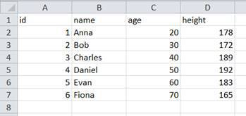
The only thing that we need to do now is to use the function read_csv to import our data into a data frame.
df = pd.read_csv( 'data.csv' )
df.set_index( 'id' , inplace = True )
print (df)
We also set the index to the id column again. This is what we have imported:
This of course, also works the other way around. By using the method to_csv , we can also save our data frame into a CSV-file.
data = { 'Name' : [ 'Anna' , 'Bob' , 'Charles' ,
'Daniel' , 'Evan' , 'Fiona' ,
'Gerald' , 'Henry' , 'India' ],
'Age' : [ 24 , 24 , 35 , 45 , 22 , 54 , 54 , 43 , 25 ],
'Height' : [ 176 , 187 , 175 , 182 , 176 ,
189 , 165 , 187 , 167 ]}
df = pd.DataFrame(data)
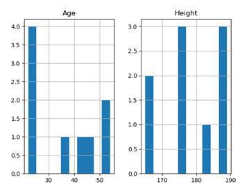
df.to_csv( 'mydf.csv' )PLOTTING DATA
Since Pandas builds on Matplotlib, we can easily visualize the data from our data frame.
data = { 'Name' : [ 'Anna' , 'Bob' , 'Charles' ,
'Daniel' , 'Evan' , 'Fiona' ,
'Gerald' , 'Henry' , 'India' ],
'Age' : [ 24 , 24 , 35 , 45 , 22 , 54 , 54 , 43 , 25 ],
'Height' : [ 176 , 187 , 175 , 182 , 176 ,
189 , 165 , 187 , 167 ]}
df = pd.DataFrame(data)
df.sort_values( by =[ 'Age' , 'Height' ])
df.hist()
plt.show()
In this example, we use the method hist to plot a histogram of our numerical columns. Without specifying anything more, this is what we end up with:
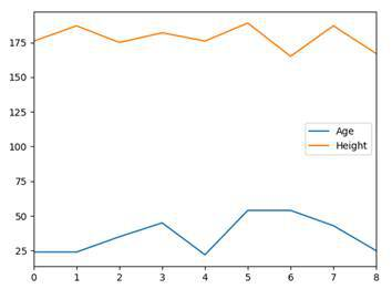
But we can also just use the function plot to plot our data frame or individual columns.
df.plot()
plt.show()
The result is the following: