Applying Logistic Regression
A case study on applying logistic regression to stock market
1:Loading Stock data
1.1:Importing libraries and data
import investpy
from datetime import datetime
from sklearn.linear_model import LogisticRegression
from sklearn.metrics import confusion_matrix
from sklearn import metrics
from scipy import stats
import numpy as np
import pandas as pd
import seaborn as sn
import matplotlib.pyplot as plt
import talib
import quandl
from sklearn.preprocessing import StandardScaler
from sklearn.metrics import accuracy_score
from sklearn.preprocessing import MinMaxScaler
import math
from sklearn.metrics import mean_squared_error
import investpy


# Set the desired date range
from_date = "2019-11-18"
to_date = "2023-11-13"
1.2:Load the data
Assuming that the data is already been downloaded in the excel sheet. We use the pandas data frame to read the data
1.2:As the commodity price also depend on exchange rate. We download that data from yahoo finance
import yfinance as yf

# Define the ticker symbol for USD/INR
symbol = "USDINR=X"

# Fetch the historical data for USD/INR
usdinr = yf.download(symbol, start=from_date, end=to_date)

# Print the retrieved data
#print(usdinr.tail())
##
[*********************100%***********************]  1 of 1 completed
1.2:As the commodity price also depend on XAGUSD, we download that data using yahoo finance
##
[*********************100%***********************]  1 of 1 completed
1.2.1: Determining position based on volume and close
1.2.2: Long positions gains
1.2.3: Short positions gains
#print(short['weekday'].value_counts())
#print(lng['weekday'].value_counts())
1.2.2: Determining Average monthly closing prices
##              Close    Open    High     Low    Volume  VolChange  CloseChange
## Date
## 2019-11-18  44.696  44.278  44.739  43.925   63510.0  26.336950     0.000623
## 2019-11-19  44.871  44.743  44.950  44.382   69630.0   0.096363     0.003915
## 2019-11-20  44.814  44.781  45.017  44.450   69850.0   0.003160    -0.001270
## 2019-11-21  44.753  44.715  44.850  44.570   45630.0  -0.346743    -0.001361
## 2019-11-22  44.489  44.744  44.985  44.460   51980.0   0.139163    -0.005899
## ...            ...     ...     ...     ...       ...        ...          ...
## 2023-08-07  71.401  72.500  72.500  71.201  127830.0  -0.121926    -0.015498
## 2023-08-08  70.398  71.497  71.497  70.200  135000.0   0.056090    -0.014047
## 2023-08-09  70.168  70.497  70.745  70.021  116800.0  -0.134815    -0.003267
## 2023-08-10  70.158  70.257  70.786  69.825  150680.0   0.290068    -0.000143
## 2023-08-11  70.150  70.250  70.500  69.805   87160.0  -0.421556    -0.000114
##
## [963 rows x 7 columns]
## Date
## 2019-11-30    44.502900
## 2019-12-31    44.983905
## 2020-01-31    46.715435
## 2020-02-29    46.769810
## 2020-03-31    42.008682
## 2020-04-30    43.175278
## 2020-05-31    46.064714
## 2020-06-30    48.667409
## 2020-07-31    55.923957
## 2020-08-31    68.698238
## 2020-09-30    65.459455
## 2020-10-31    61.675571
## 2020-11-30    62.012955
## 2020-12-31    65.897045
## 2021-01-31    67.186000
## 2021-02-28    69.205200
## 2021-03-31    66.495957
## 2021-04-30    67.700095
## 2021-05-31    71.556381
## 2021-06-30    70.013318
## 2021-07-31    68.518000
## 2021-08-31    63.957364
## 2021-09-30    62.362182
## 2021-10-31    63.489333
## 2021-11-30    64.592091
## 2021-12-31    61.979783
## 2022-01-31    62.549050
## 2022-02-28    63.447050
## 2022-03-31    68.742739
## 2022-04-30    67.053300
## 2022-05-31    61.769045
## 2022-06-30    61.141136
## 2022-07-31    56.920238
## 2022-08-31    57.243818
## 2022-09-30    56.261182
## 2022-10-31    58.740095
## 2022-11-30    61.312727
## 2022-12-31    68.004727
## 2023-01-31    68.816714
## 2023-02-28    66.319550
## 2023-03-31    67.243826
## 2023-04-30    74.628737
## 2023-05-31    73.751652
## 2023-06-30    71.120091
## 2023-07-31    73.584143
## 2023-08-31    71.584333
## Freq: M, Name: Close, dtype: float64
1.2.3: Technical moving averages
1.2.4: Determining the z-scores
1.2.5: Determining the daily support and resistance levels
#Pivot Points, Supports and Resistances
def PPSR(df):
    PP = pd.Series((df['High'] + df['Low'] + df['Close']) / 3)
    R1 = pd.Series(2 * PP - df['Low'])
    S1 = pd.Series(2 * PP - df['High'])
    R2 = pd.Series(PP + df['High'] - df['Low'])
    S2 = pd.Series(PP - df['High'] + df['Low'])
    R3 = pd.Series(df['High'] + 2 * (PP - df['Low']))
    S3 = pd.Series(df['Low'] - 2 * (df['High'] - PP))
    psr = {'PP':PP, 'R1':R1, 'S1':S1, 'R2':R2, 'S2':S2, 'R3':R3, 'S3':S3}
    psrdf = pd.DataFrame(psr)
    psrdf = psrdf*1000
    #df = df.join(PSR)
    return psrdf.round().tail()

#PPSR(df)
1.2.6: Fibonnacci retracement levels
## Retracement levels for rising price
##                               0
## 0             {'min': [69.805]}
## 1  {'level5(61.8)': [70.07049]}
## 2     {'level4(50)': [70.1525]}
## 3  {'level3(38.2)': [70.23451]}
## 4  {'level2(23.6)': [70.33598]}
## 5              {'zero': [70.5]}
## Retracement levels for falling price
As we can see, we now have a data frame with all the entries from start date to end date. We have multiple columns here and not only the closing stock price of the respective day. Let’s take a quick look at the individual columns and their meaning.
Open: That’s the share price the stock had when the markets opened that day.
Close: That’s the share price the stock had when the markets closed that day.
High: That’s the highest share price that the stock had that day.
Low: That’s the lowest share price that the stock had that day.
Volume: Amount of shares that changed hands that day.
1.3:Reading individual values
Since our data is stored in a Pandas data frame, we can use the indexing we already know, to get individual values. For example, we could only print the closing values using print (df[ 'Close' ])
Also, we can go ahead and print the closing value of a specific date that we are interested in. This is possible because the date is our index column.
print (df[ 'Close' ][ '2020-07-14' ])
But we could also use simple indexing to access certain positions.
print (df[ 'Close' ][ 5 ])
## 44.245
Here we printed the closing price of the fifth entry.
2:Graphical Visualization
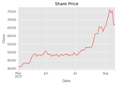
Even though tables are nice and useful, we want to visualize our financial data, in order to get a better overview. We want to look at the development of the share price.
Actually plotting our share price curve with Pandas and Matplotlib is very simple. Since Pandas builds on top of Matplotlib, we can just select the column we are interested in and apply the plot method. The results are amazing. Since the date is the index of our data frame, Matplotlib uses it for the x-axis. The y-values are then our adjusted close values.
2.1:CandleStick Charts
The best way to visualize stock data is to use so-called candlestick charts . This type of chart gives us information about four different values at the same time, namely the high, the low, the open and the close value. In order to plot candlestick charts, we will need to import a function of the MPL-Finance library.
import mplfinance as fplt
We are importing the candlestick_ohlc function. Notice that there also exists a candlestick_ochl function that takes in the data in a different order. Also, for our candlestick chart, we will need a different date format provided by Matplotlib. Therefore, we need to import the respective module as well. We give it the alias mdates .
import matplotlib.dates as mdates
2.2: Preparing the data for CandleStick charts
Now in order to plot our stock data, we need to select the four columns in the right order.
df1 = df[[ 'Open' , 'High' , 'Low' , 'Close' ]]
Now, we have our columns in the right order but there is still a problem. Our date doesn’t have the right format and since it is the index, we cannot manipulate it. Therefore, we need to reset the index and then convert our datetime to a number.
df1.reset_index( inplace = True )
df1[ 'Date' ] = df1[ 'Date' ].map(mdates.date2num)
## <string>:1: SettingWithCopyWarning:
## A value is trying to be set on a copy of a slice from a DataFrame.
## Try using .loc[row_indexer,col_indexer] = value instead
##
## See the caveats in the documentation: https://pandas.pydata.org/pandas-docs/stable/user_guide/indexing.html#returning-a-view-versus-a-copy
For this, we use the reset_index function so that we can manipulate our Date column. Notice that we are using the inplace parameter to replace the data frame by the new one. After that, we map the date2num function of the matplotlib.dates module on all of our values. That converts our dates into numbers that we can work with.
2.3:Plotting the data
Now we can start plotting our graph. For this, we just define a subplot (because we need to pass one to our function) and call our candlestick_ohlc function.
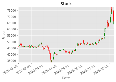
One candlestick gives us the information about all four values of one specific day. The highest point of the stick is the high and the lowest point is the low of that day. The colored area is the difference between the open and the close price. If the stick is green, the close value is at the top and the open value at the bottom, since the close must be higher than the open. If it is red, it is the other way around.
***2.4:Analysis and Statistics ***
Now let’s get a little bit deeper into the numbers here and away from the visual. From our data we can derive some statistical values that will help us to analyze it.
PERCENTAGE CHANGE
One value that we can calculate is the percentage change of that day. This means by how many percent the share price increased or decreased that day.
The calculation is quite simple. We create a new column with the name PCT_Change and the values are just the difference of the closing and opening values divided by the opening values. Since the open value is the beginning value of that day, we take it as a basis. We could also multiply the result by 100 to get the actual percentage.
*** HIGH LOW PERCENTAGE ***
Another interesting statistic is the high low percentage. Here we just calculate the difference between the highest and the lowest value and divide it by the closing value.
By doing that we can get a feeling of how volatile the stock is.
These statistical values can be used with many others to get a lot of valuable information about specific stocks. This improves the decision making
*** MOVING AVERAGE ***
we are going to derive the different moving averages . It is the arithmetic mean of all the values of the past n days. Of course this is not the only key statistic that we can derive, but it is the one we are going to use now. We can play around with other functions as well.
What we are going to do with this value is to include it into our data frame and to compare it with the share price of that day.
For this, we will first need to create a new column. Pandas does this automatically when we assign values to a column name. This means that we don’t have to explicitly define that we are creating a new column.
##              Close  5d_ma  20d_ma  50d_ma  ...  20d_ema  50d_ema  100d_ema  200d_ema
## Date                                       ...
## 2023-08-03  72.577  73.74   74.09   72.30  ...    73.63    72.88     71.81     69.52
## 2023-08-04  72.525  73.45   74.15   72.33  ...    73.52    72.87     71.82     69.55
## 2023-08-07  71.401  72.68   74.15   72.33  ...    73.32    72.81     71.81     69.57
## 2023-08-08  70.398  71.98   74.11   72.32  ...    73.04    72.71     71.79     69.58
## 2023-08-09  70.168  71.41   73.95   72.28  ...    72.77    72.61     71.75     69.58
## 2023-08-10  70.158  70.93   73.71   72.23  ...    72.52    72.52     71.72     69.59
## 2023-08-11  70.150  70.46   73.43   72.19  ...    72.29    72.42     71.69     69.59
##
## [7 rows x 11 columns]
Here we define a three new columns with the name 20d_ma, 50d_ma, 100d_ma,200d_ma . We now fill this column with the mean values of every n entries. The rolling function stacks a specific amount of entries, in order to make a statistical calculation possible. The window parameter is the one which defines how many entries we are going to stack. But there is also the min_periods parameter. This one defines how many entries we need to have as a minimum in order to perform the calculation. This is relevant because the first entries of our data frame won’t have a n entries previous to them. By setting this value to zero we start the calculations already with the first number, even if there is not a single previous value. This has the effect that the first value will be just the first number, the second one will be the mean of the first two numbers and so on, until we get to a b values.
By using the mean function, we are obviously calculating the arithmetic mean. However, we can use a bunch of other functions like max, min or median if we like to.
*** Standard Deviation ***
The variability of the closing stock prices determinies how vo widely prices are dispersed from the average price. If the prices are trading in narrow trading range the standard deviation will return a low value that indicates low volatility. If the prices are trading in wide trading range the standard deviation will return high value that indicates high volatility.
## Date
## 2023-08-03    1.010715
## 2023-08-04    0.959772
## 2023-08-07    1.252779
## 2023-08-08    1.584938
## 2023-08-09    1.380740
## 2023-08-10    1.240766
## 2023-08-11    1.113489
## Name: Std_dev, dtype: float64
*** Relative Strength Index ***
The relative strength index is a indicator of mementum used in technical analysis that measures the magnitude of current price changes to know overbought or oversold conditions in the price of a stock or other asset. If RSI is above 70 then it is overbought. If RSI is below 30 then it is oversold condition.
##                   RSI
## Date
## 2023-08-07  34.201742
## 2023-08-08  29.425557
## 2023-08-09  28.402343
## 2023-08-10  28.354117
## 2023-08-11  28.310853
*** Average True range ***
##                     ATR     20dayEMA    ATRdiff
## Date
## 2023-08-07  1293.506955  1258.339475  35.167479
## 2023-08-08  1293.756458  1261.712521  32.043937
## 2023-08-09  1253.059568  1260.888431  -7.828862
## 2023-08-10  1232.198170  1258.156025 -25.957854
## 2023-08-11  1193.826872  1252.029439 -58.202566
*** Wiliams %R ***
Williams %R, or just %R, is a technical analysis oscillator showing the current closing price in relation to the high and low of the past N days.The oscillator is on a negative scale, from −100 (lowest) up to 0 (highest). A value of −100 means the close today was the lowest low of the past N days, and 0 means today’s close was the highest high of the past N days.
##             Williams %R
## Date
## 2023-08-03   -85.826972
## 2023-08-04   -82.134293
## 2023-08-07   -95.119571
## 2023-08-08   -96.116886
## 2023-08-09   -97.065868
## 2023-08-10   -93.169231
## 2023-08-11   -89.133858
Readings below -80 represent oversold territory and readings above -20 represent overbought.
*** ADX ***
ADX is used to quantify trend strength. ADX calculations are based on a moving average of price range expansion over a given period of time. The average directional index (ADX) is used to determine when the price is trending strongly.
0-25: Absent or Weak Trend
25-50: Strong Trend
50-75: Very Strong Trend
75-100: Extremely Strong Trend
##                   ADX
## Date
## 2023-08-03  22.356323
## 2023-08-04  23.321120
## 2023-08-07  25.614017
## 2023-08-08  29.536658
## 2023-08-09  33.200753
## 2023-08-10  36.689600
## 2023-08-11  39.718986
##                    CCI
## Date
## 2023-08-03 -187.615350
## 2023-08-04 -156.219131
## 2023-08-07 -170.734667
## 2023-08-08 -180.249253
## 2023-08-09 -155.559619
## 2023-08-10 -126.324384
## 2023-08-11 -108.824802
##                  ROC
## Date
## 2023-08-03 -3.595718
## 2023-08-04 -3.091971
## 2023-08-07 -3.493904
## 2023-08-08 -5.683280
## 2023-08-09 -6.679080
## 2023-08-10 -4.763327
## 2023-08-11 -5.162974
*** MACD ***
Moving Average Convergence Divergence (MACD) is a trend-following momentum indicator that shows the relationship between two moving averages of a security’s price. The MACD is calculated by subtracting the 26-period Exponential Moving Average (EMA) from the 12-period EMA.
##             MACD_IND
## Date
## 2023-08-07 -0.434200
## 2023-08-08 -0.537966
## 2023-08-09 -0.593049
## 2023-08-10 -0.599340
## 2023-08-11 -0.573226
##              Close    Open    High  ...      MACD  Signal Line  MACD_IND
## Date                                ...
## 2023-08-07  71.401  72.500  72.500  ...  0.091686     0.525886 -0.434200
## 2023-08-08  70.398  71.497  71.497  ... -0.146571     0.391394 -0.537966
## 2023-08-09  70.168  70.497  70.745  ... -0.349917     0.243132 -0.593049
## 2023-08-10  70.158  70.257  70.786  ... -0.506043     0.093297 -0.599340
## 2023-08-11  70.150  70.250  70.500  ... -0.623236    -0.050009 -0.573226
##
## [5 rows x 42 columns]
*** Bollinger Bands ***
Bollinger Bands are a type of statistical chart characterizing the prices and volatility over time of a financial instrument or commodity.
## 77390.0 73430.0 69460.0
In case we choose another value than zero for our min_periods parameter, we will end up with a couple of NaN-Values . These are not a number values and they are useless. Therefore, we would want to delete the entries that have such values.
We do this by using the dropna function. If we would have had any entries with NaN values in any column, they would now have been deleted
3: Predicting the movement of stock
To predict the movement of the stock we use 5 lag returns as the dependent variables. The first leg is return yesterday, leg2 is return day before yesterday and so on. The dependent variable is whether the prices went up or down on that day. Other variables include the technical indicators which along with 5 lag returns are used to predict the movement of stock using logistic regression.
3.1: Creating lag returns
3.2: Creating returns dataframe
3.2: create the lagged percentage returns columns
##                Today      Lag1      Lag2  ...     Lag13     Lag14     Lag15
## Date                                      ...
## 2023-07-31  1.743974  0.409953 -2.025535  ...  3.131715 -0.254941  0.061672
## 2023-08-01 -1.824367  1.743974  0.409953  ...  2.222313  3.131715 -0.254941
## 2023-08-02 -1.204558 -1.824367  1.743974  ...  0.879191  2.222313  3.131715
## 2023-08-03 -0.574004 -1.204558 -1.824367  ... -0.492546  0.879191  2.222313
## 2023-08-04 -0.071648 -0.574004 -1.204558  ...  0.717926 -0.492546  0.879191
## 2023-08-07 -1.549810 -0.071648 -0.574004  ...  0.368921  0.717926 -0.492546
## 2023-08-08 -1.404742 -1.549810 -0.071648  ... -1.172270  0.368921  0.717926
## 2023-08-09 -0.326714 -1.404742 -1.549810  ... -0.591095 -1.172270  0.368921
## 2023-08-10 -0.014252 -0.326714 -1.404742  ... -1.139780 -0.591095 -1.172270
## 2023-08-11 -0.011403 -0.014252 -0.326714  ...  0.883951 -1.139780 -0.591095
##
## [10 rows x 16 columns]
3.3: “Direction” column (+1 or -1) indicating an up/down day
***3.4: Create the dependent and independent variables ***
## <string>:1: SettingWithCopyWarning:
## A value is trying to be set on a copy of a slice from a DataFrame.
## Try using .loc[row_indexer,col_indexer] = value instead
##
## See the caveats in the documentation: https://pandas.pydata.org/pandas-docs/stable/user_guide/indexing.html#returning-a-view-versus-a-copy
##                 Lag1      Lag2      Lag3  ...         DX  Open-Close  Open-Open
## Date                                      ...
## 2023-08-07 -0.071648 -0.574004 -1.204558  ...  16.639989      -0.025     -0.020
## 2023-08-08 -1.549810 -0.071648 -0.574004  ...  26.314423       0.096     -1.003
## 2023-08-09 -1.404742 -1.549810 -0.071648  ...  27.925271       0.099     -1.000
## 2023-08-10 -0.326714 -1.404742 -1.549810  ...  29.736565       0.089     -0.240
## 2023-08-11 -0.014252 -0.326714 -1.404742  ...  29.930072       0.092     -0.007
##
## [5 rows x 34 columns]
3.5: Create training and test sets
##                 Lag1      Lag2      Lag3  ...         DX  Open-Close  Open-Open
## Date                                      ...
## 2023-08-07 -0.071648 -0.574004 -1.204558  ...  16.639989      -0.025     -0.020
## 2023-08-08 -1.549810 -0.071648 -0.574004  ...  26.314423       0.096     -1.003
## 2023-08-09 -1.404742 -1.549810 -0.071648  ...  27.925271       0.099     -1.000
## 2023-08-10 -0.326714 -1.404742 -1.549810  ...  29.736565       0.089     -0.240
## 2023-08-11 -0.014252 -0.326714 -1.404742  ...  29.930072       0.092     -0.007
##
## [5 rows x 34 columns]
***3.6: Create model ***
3.7: train the model on the training set
<style>#sk-container-id-1 {color: black;background-color: white;}#sk-container-id-1 pre{padding: 0;}#sk-container-id-1 div.sk-toggleable {background-color: white;}#sk-container-id-1 label.sk-toggleable__label {cursor: pointer;display: block;width: 100%;margin-bottom: 0;padding: 0.3em;box-sizing: border-box;text-align: center;}#sk-container-id-1 label.sk-toggleable__label-arrow:before {content: "▸";float: left;margin-right: 0.25em;color: #696969;}#sk-container-id-1 label.sk-toggleable__label-arrow:hover:before {color: black;}#sk-container-id-1 div.sk-estimator:hover label.sk-toggleable__label-arrow:before {color: black;}#sk-container-id-1 div.sk-toggleable__content {max-height: 0;max-width: 0;overflow: hidden;text-align: left;background-color: #f0f8ff;}#sk-container-id-1 div.sk-toggleable__content pre {margin: 0.2em;color: black;border-radius: 0.25em;background-color: #f0f8ff;}#sk-container-id-1 input.sk-toggleable__control:checked~div.sk-toggleable__content {max-height: 200px;max-width: 100%;overflow: auto;}#sk-container-id-1 input.sk-toggleable__control:checked~label.sk-toggleable__label-arrow:before {content: "▾";}#sk-container-id-1 div.sk-estimator input.sk-toggleable__control:checked~label.sk-toggleable__label {background-color: #d4ebff;}#sk-container-id-1 div.sk-label input.sk-toggleable__control:checked~label.sk-toggleable__label {background-color: #d4ebff;}#sk-container-id-1 input.sk-hidden--visually {border: 0;clip: rect(1px 1px 1px 1px);clip: rect(1px, 1px, 1px, 1px);height: 1px;margin: -1px;overflow: hidden;padding: 0;position: absolute;width: 1px;}#sk-container-id-1 div.sk-estimator {font-family: monospace;background-color: #f0f8ff;border: 1px dotted black;border-radius: 0.25em;box-sizing: border-box;margin-bottom: 0.5em;}#sk-container-id-1 div.sk-estimator:hover {background-color: #d4ebff;}#sk-container-id-1 div.sk-parallel-item::after {content: "";width: 100%;border-bottom: 1px solid gray;flex-grow: 1;}#sk-container-id-1 div.sk-label:hover label.sk-toggleable__label {background-color: #d4ebff;}#sk-container-id-1 div.sk-serial::before {content: "";position: absolute;border-left: 1px solid gray;box-sizing: border-box;top: 0;bottom: 0;left: 50%;z-index: 0;}#sk-container-id-1 div.sk-serial {display: flex;flex-direction: column;align-items: center;background-color: white;padding-right: 0.2em;padding-left: 0.2em;position: relative;}#sk-container-id-1 div.sk-item {position: relative;z-index: 1;}#sk-container-id-1 div.sk-parallel {display: flex;align-items: stretch;justify-content: center;background-color: white;position: relative;}#sk-container-id-1 div.sk-item::before, #sk-container-id-1 div.sk-parallel-item::before {content: "";position: absolute;border-left: 1px solid gray;box-sizing: border-box;top: 0;bottom: 0;left: 50%;z-index: -1;}#sk-container-id-1 div.sk-parallel-item {display: flex;flex-direction: column;z-index: 1;position: relative;background-color: white;}#sk-container-id-1 div.sk-parallel-item:first-child::after {align-self: flex-end;width: 50%;}#sk-container-id-1 div.sk-parallel-item:last-child::after {align-self: flex-start;width: 50%;}#sk-container-id-1 div.sk-parallel-item:only-child::after {width: 0;}#sk-container-id-1 div.sk-dashed-wrapped {border: 1px dashed gray;margin: 0 0.4em 0.5em 0.4em;box-sizing: border-box;padding-bottom: 0.4em;background-color: white;}#sk-container-id-1 div.sk-label label {font-family: monospace;font-weight: bold;display: inline-block;line-height: 1.2em;}#sk-container-id-1 div.sk-label-container {text-align: center;}#sk-container-id-1 div.sk-container {/* jupyter's `normalize.less` sets `[hidden] { display: none; }` but bootstrap.min.css set `[hidden] { display: none !important; }` so we also need the `!important` here to be able to override the default hidden behavior on the sphinx rendered scikit-learn.org. See: https://github.com/scikit-learn/scikit-learn/issues/21755 */display: inline-block !important;position: relative;}#sk-container-id-1 div.sk-text-repr-fallback {display: none;}</style><div id="sk-container-id-1" class="sk-top-container"><div class="sk-text-repr-fallback"><pre>LogisticRegression(max_iter=1000000)</pre><b>In a Jupyter environment, please rerun this cell to show the HTML representation or trust the notebook. <br />On GitHub, the HTML representation is unable to render, please try loading this page with nbviewer.org.</b></div><div class="sk-container" hidden><div class="sk-item"><div class="sk-estimator sk-toggleable"><input class="sk-toggleable__control sk-hidden--visually" id="sk-estimator-id-1" type="checkbox" checked><label for="sk-estimator-id-1" class="sk-toggleable__label sk-toggleable__label-arrow">LogisticRegression</label><div class="sk-toggleable__content"><pre>LogisticRegression(max_iter=1000000)</pre></div></div></div></div></div>
3.8: make an array of predictions on the test set
3.9: output the hit-rate and the confusion matrix for the model
##
## Train Accuracy: 91.60%
## Test Accuracy: 69.89%
## [[192  74]
##  [122 263]]
***3.10: Predict movement of stock for tomorrow. ***
##             y_test  y_pred
## Date
## 2023-08-07      -1      -1
## 2023-08-08      -1      -1
## 2023-08-09      -1      -1
## 2023-08-10      -1      -1
## 2023-08-11      -1      -1
## [-1]
1.2.2: Determining Average monthly closing prices
1.2.3: Technical moving averages
1.2.4: Determining the z-scores
1.2.5: Determining the daily support and resistance levels
1.2.6: Fibonnacci retracement levels
As we can see, we now have a data frame with all the entries from start date to end date. We have multiple columns here and not only the closing stock price of the respective day. Let’s take a quick look at the individual columns and their meaning.
Open: That’s the share price the stock had when the markets opened that day.
Close: That’s the share price the stock had when the markets closed that day.
High: That’s the highest share price that the stock had that day.
Low: That’s the lowest share price that the stock had that day.
Volume: Amount of shares that changed hands that day.
1.3:Reading individual values
Since our data is stored in a Pandas data frame, we can use the indexing we already know, to get individual values. For example, we could only print the closing values using print (df[ 'Close' ])
Also, we can go ahead and print the closing value of a specific date that we are interested in. This is possible because the date is our index column.
But we could also use simple indexing to access certain positions.
Here we printed the closing price of the fifth entry.
2:Graphical Visualization
Even though tables are nice and useful, we want to visualize our financial data, in order to get a better overview. We want to look at the development of the share price.
Actually plotting our share price curve with Pandas and Matplotlib is very simple. Since Pandas builds on top of Matplotlib, we can just select the column we are interested in and apply the plot method. The results are amazing. Since the date is the index of our data frame, Matplotlib uses it for the x-axis. The y-values are then our adjusted close values.
2.1:CandleStick Charts
The best way to visualize stock data is to use so-called candlestick charts . This type of chart gives us information about four different values at the same time, namely the high, the low, the open and the close value. In order to plot candlestick charts, we will need to import a function of the MPL-Finance library.
We are importing the candlestick_ohlc function. Notice that there also exists a candlestick_ochl function that takes in the data in a different order. Also, for our candlestick chart, we will need a different date format provided by Matplotlib. Therefore, we need to import the respective module as well. We give it the alias mdates .
2.2: Preparing the data for CandleStick charts
Now in order to plot our stock data, we need to select the four columns in the right order.
df1 = df[[ 'Open' , 'High' , 'Low' , 'Close' ]]
Now, we have our columns in the right order but there is still a problem. Our date doesn’t have the right format and since it is the index, we cannot manipulate it. Therefore, we need to reset the index and then convert our datetime to a number.
For this, we use the reset_index function so that we can manipulate our Date column. Notice that we are using the inplace parameter to replace the data frame by the new one. After that, we map the date2num function of the matplotlib.dates module on all of our values. That converts our dates into numbers that we can work with.
2.3:Plotting the data
Now we can start plotting our graph. For this, we just define a subplot (because we need to pass one to our function) and call our candlestick_ohlc function.
One candlestick gives us the information about all four values of one specific day. The highest point of the stick is the high and the lowest point is the low of that day. The colored area is the difference between the open and the close price. If the stick is green, the close value is at the top and the open value at the bottom, since the close must be higher than the open. If it is red, it is the other way around.
***2.4:Analysis and Statistics ***
Now let’s get a little bit deeper into the numbers here and away from the visual. From our data we can derive some statistical values that will help us to analyze it.
PERCENTAGE CHANGE
One value that we can calculate is the percentage change of that day. This means by how many percent the share price increased or decreased that day.
The calculation is quite simple. We create a new column with the name PCT_Change and the values are just the difference of the closing and opening values divided by the opening values. Since the open value is the beginning value of that day, we take it as a basis. We could also multiply the result by 100 to get the actual percentage.
*** HIGH LOW PERCENTAGE ***
Another interesting statistic is the high low percentage. Here we just calculate the difference between the highest and the lowest value and divide it by the closing value.
By doing that we can get a feeling of how volatile the stock is.
These statistical values can be used with many others to get a lot of valuable information about specific stocks. This improves the decision making
*** MOVING AVERAGE ***
we are going to derive the different moving averages . It is the arithmetic mean of all the values of the past n days. Of course this is not the only key statistic that we can derive, but it is the one we are going to use now. We can play around with other functions as well.
What we are going to do with this value is to include it into our data frame and to compare it with the share price of that day.
For this, we will first need to create a new column. Pandas does this automatically when we assign values to a column name. This means that we don’t have to explicitly define that we are creating a new column.
Here we define a three new columns with the name 20d_ma, 50d_ma, 100d_ma,200d_ma . We now fill this column with the mean values of every n entries. The rolling function stacks a specific amount of entries, in order to make a statistical calculation possible. The window parameter is the one which defines how many entries we are going to stack. But there is also the min_periods parameter. This one defines how many entries we need to have as a minimum in order to perform the calculation. This is relevant because the first entries of our data frame won’t have a n entries previous to them. By setting this value to zero we start the calculations already with the first number, even if there is not a single previous value. This has the effect that the first value will be just the first number, the second one will be the mean of the first two numbers and so on, until we get to a b values.
By using the mean function, we are obviously calculating the arithmetic mean. However, we can use a bunch of other functions like max, min or median if we like to.
*** Standard Deviation ***
The variability of the closing stock prices determinies how vo widely prices are dispersed from the average price. If the prices are trading in narrow trading range the standard deviation will return a low value that indicates low volatility. If the prices are trading in wide trading range the standard deviation will return high value that indicates high volatility.
*** Relative Strength Index ***
The relative strength index is a indicator of mementum used in technical analysis that measures the magnitude of current price changes to know overbought or oversold conditions in the price of a stock or other asset. If RSI is above 70 then it is overbought. If RSI is below 30 then it is oversold condition.
*** Average True range ***
*** Wiliams %R ***
Williams %R, or just %R, is a technical analysis oscillator showing the current closing price in relation to the high and low of the past N days.The oscillator is on a negative scale, from −100 (lowest) up to 0 (highest). A value of −100 means the close today was the lowest low of the past N days, and 0 means today’s close was the highest high of the past N days.
Readings below -80 represent oversold territory and readings above -20 represent overbought.
*** ADX ***
ADX is used to quantify trend strength. ADX calculations are based on a moving average of price range expansion over a given period of time. The average directional index (ADX) is used to determine when the price is trending strongly.
0-25: Absent or Weak Trend
25-50: Strong Trend
50-75: Very Strong Trend
75-100: Extremely Strong Trend
*** MACD ***
Moving Average Convergence Divergence (MACD) is a trend-following momentum indicator that shows the relationship between two moving averages of a security’s price. The MACD is calculated by subtracting the 26-period Exponential Moving Average (EMA) from the 12-period EMA.
*** Bollinger Bands ***
Bollinger Bands are a type of statistical chart characterizing the prices and volatility over time of a financial instrument or commodity.
In case we choose another value than zero for our min_periods parameter, we will end up with a couple of NaN-Values . These are not a number values and they are useless. Therefore, we would want to delete the entries that have such values.
We do this by using the dropna function. If we would have had any entries with NaN values in any column, they would now have been deleted
3: Predicting the movement of stock
To predict the movement of the stock we use 5 lag returns as the dependent variables. The first leg is return yesterday, leg2 is return day before yesterday and so on. The dependent variable is whether the prices went up or down on that day. Other variables include the technical indicators which along with 5 lag returns are used to predict the movement of stock using logistic regression.
3.1: Creating lag returns
3.2: Creating returns dataframe
3.2: create the lagged percentage returns columns
3.3: “Direction” column (+1 or -1) indicating an up/down day
***3.4: Create the dependent and independent variables ***
3.5: Create training and test sets
***3.6: Create model ***
3.7: train the model on the training set
3.8: make an array of predictions on the test set
3.9: output the hit-rate and the confusion matrix for the model
***3.10: Predict movement of stock for tomorrow. ***